ATGC数量柱状图 |Nature

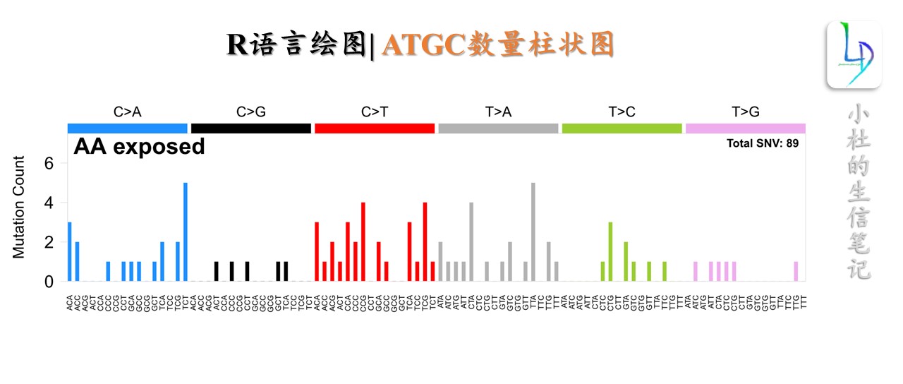
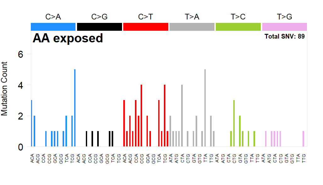
原文教程：R语言绘制 | ATGC数量柱状图 |Nature

本期教程

获得本教程Data and Code，请在后台回复：20240812。

2022年教程总汇

2023年教程总汇

Code

1. 导入R包

library(RColorBrewer)
library(pheatmap)
library(tidyverse)
library(viridis)
library(reshape2)
filter = dplyr::filter

2. 导入对应数据

input <- read.csv(file="data_Spectra_Input.csv")

head(input)

> head(input)
  sampleID   chr       pos ref mut type   effect     gene trinuc_ref sub trinuc_ref_py firstbase thirdbase py_ref
1 PD46845a  chr2 157766005   C   A  Sub missense    ACVR1        CCT C>A           CCT         C         T      C
2 PD51536a chr14 104780108   A   C  Sub missense     AKT1        GAG T>G           CTC         C         C      T
3 PD42673a chr14 104780214   C   T  Sub missense     AKT1        TCC C>T           TCC         T         C      C
4 PD46732a  chr5 112821985   G   T  Sub nonsense      APC        TGA C>A           TCA         T         A      C
5 PD51821a  chr5 112838196   G   T  Sub nonsense      APC        AGA C>A           TCT         T         T      C
6 PD51600a chr19  46921195   C   A  Sub nonsense ARHGAP35        ACC C>A           ACC         A         C      C
  py_alt context
1      A C[C>A]T
2      G C[T>G]C
3      T T[C>T]C
4      A T[C>A]A
5      A T[C>A]T
6      A A[C>A]C

AA_exposed <- read.csv(file="data_AA_Input.csv")
head(AA_exposed)

> head(AA_exposed)
    Sample Country SBS22a SBS22b SBS22a_relative SBS22b_relative
1 PD37463a Romania   6878   8024          0.3119          0.3639
2 PD37464a Romania    660   1049          0.1196          0.1901
3 PD37466a Romania   1349   1301          0.2088          0.2014
4 PD37469a Romania      0   2539          0.0000          0.3993
5 PD37484a Romania   3718   7772          0.2712          0.5670
6 PD42572a  Serbia   4015   3463          0.3788          0.3268

3. 提取、计算、分析

### 绘图函数
plot_driver_spectra = function(input, plot_title) {
  #Collect Data
  mutations = input
  #Define contexts
  matrix_contexts <- c('A[C>A]A', 'A[C>A]C', 'A[C>A]G', 'A[C>A]T', 'C[C>A]A', 'C[C>A]C', 'C[C>A]G', 'C[C>A]T',
                       'G[C>A]A', 'G[C>A]C', 'G[C>A]G', 'G[C>A]T', 'T[C>A]A', 'T[C>A]C', 'T[C>A]G', 'T[C>A]T',
                       'A[C>G]A', 'A[C>G]C', 'A[C>G]G', 'A[C>G]T', 'C[C>G]A', 'C[C>G]C', 'C[C>G]G', 'C[C>G]T', 
                       'G[C>G]A', 'G[C>G]C', 'G[C>G]G', 'G[C>G]T', 'T[C>G]A', 'T[C>G]C', 'T[C>G]G', 'T[C>G]T',
                       'A[C>T]A', 'A[C>T]C', 'A[C>T]G', 'A[C>T]T', 'C[C>T]A', 'C[C>T]C', 'C[C>T]G', 'C[C>T]T',
                       'G[C>T]A', 'G[C>T]C', 'G[C>T]G', 'G[C>T]T', 'T[C>T]A', 'T[C>T]C', 'T[C>T]G', 'T[C>T]T',
                       'A[T>A]A', 'A[T>A]C', 'A[T>A]G', 'A[T>A]T', 'C[T>A]A', 'C[T>A]C', 'C[T>A]G', 'C[T>A]T',
                       'G[T>A]A', 'G[T>A]C', 'G[T>A]G', 'G[T>A]T', 'T[T>A]A', 'T[T>A]C', 'T[T>A]G', 'T[T>A]T',
                       'A[T>C]A', 'A[T>C]C', 'A[T>C]G', 'A[T>C]T', 'C[T>C]A', 'C[T>C]C', 'C[T>C]G', 'C[T>C]T',
                       'G[T>C]A', 'G[T>C]C', 'G[T>C]G', 'G[T>C]T', 'T[T>C]A', 'T[T>C]C', 'T[T>C]G', 'T[T>C]T',
                       'A[T>G]A', 'A[T>G]C', 'A[T>G]G', 'A[T>G]T', 'C[T>G]A', 'C[T>G]C', 'C[T>G]G', 'C[T>G]T',
                       'G[T>G]A', 'G[T>G]C', 'G[T>G]G', 'G[T>G]T', 'T[T>G]A', 'T[T>G]C', 'T[T>G]G', 'T[T>G]T')
  #Count Occurances
  freq=c(table(mutations$context))
  mutations_ctx=data.frame(ctxt=matrix_contexts,counts=freq[matrix_contexts])
  mutations_ctx <- tibble::column_to_rownames(mutations_ctx,"ctxt")
  mutations_ctx[is.na(mutations_ctx)] = 0
  rownames(mutations_ctx) <- NULL
  
  #Plot!
  # Specify Context Type
  sig_cat = c("C>A","C>G","C>T","T>A","T>C","T>G")
  ctx_vec = paste(rep(c("A","C","G","T"),each=4),rep(c("A","C","G","T"),times=4),sep="-")
  full_vec = paste(rep(sig_cat,each=16),rep(ctx_vec,times=6),sep=",")
  snv_context = paste(substr(full_vec,5,5), substr(full_vec,1,1), substr(full_vec,7,7), sep="")
  # Specify Vectors for plot colours
  col_vec_num <- rep(16,6)
  col_vec = rep(c("dodgerblue","black","red","grey70","olivedrab3","plum2"),each=16)
  # Convert to matrix
  sig_plot <- as.matrix(mutations_ctx)
  # Set up Signature Names and title
  sig_title <- colnames(sig_plot)
  # Set up Counts
  sample_counts <- colSums(mutations_ctx)
  # Set par settings
  par(xaxs='i', cex = 1, xpd = FALSE)
  #  define maxy
  max_prob <- sig_plot[,1];maxy = max(max_prob)
  #  call empty plot
  b = barplot(sig_plot[,1], col = NA, border = NA, axes = FALSE, las = 2, ylim=c(0,1.5*maxy), 
              names.arg = snv_context, cex.lab = 1.3, cex.names = 0.70, cex.axis = 2, 
              space = 1, ylab = "Mutation Count")  
  # add axis
  axis(2, at = pretty(0:(1.5*maxy), n = 3), col = 'grey90', las = 1, cex.axis = 1.5)
  # call columns
  b = barplot(sig_plot[,1], axes = FALSE, col=col_vec, add = T, border = NA, space = 1)
  # add box surronding plot
  box(lty = 1, col = 'grey90')
  # add title
  title(plot_title, line = -1.5, adj = 0.01, cex.main = 2)
  title(paste0("Total SNV: ", sample_counts), line = -1, adj = 0.99, cex.main = 1)
  # add rectangles and annotations on top of the plot
  par(xpd = NA)
  for (j in 1:length(sig_cat)) {
    xpos = b[c(sum(col_vec_num[1:j])-col_vec_num[j]+1,sum(col_vec_num[1:j]))]
    rect(xpos[1]-0.5, maxy*1.5, xpos[2]+0.5, maxy*1.6, border=NA, col=unique(col_vec)[j])
    text(x=mean(xpos), pos=3, y=maxy*1.6, label=sig_cat[j], cex = 1.25)
  } 
}

5. 提取、计算、分析

#Subset only for cases with >10% COSMIC attribution to either AA signatures

input_AA <- subset(input, (sampleID %in% AA_exposed$Sample))
input_nonAA <-subset(input, (!sampleID %in% AA_exposed$Sample))

6. 绘图

plot_driver_spectra(input_AA,"AA exposed")

获得本教程Data and Code，请在后台回复：20240812。

若我们的教程对你有所帮助，请点赞+收藏+转发，这是对我们最大的支持。

往期部分文章

1. 最全WGCNA教程（替换数据即可出全部结果与图形）

• WGCNA分析 | 全流程分析代码 | 代码一

• WGCNA分析 | 全流程分析代码 | 代码二

• WGCNA分析 | 全流程代码分享 | 代码三

• WGCNA分析 | 全流程分析代码 | 代码四

• WGCNA分析 | 全流程分析代码 | 代码五(最新版本)

---

2. 精美图形绘制教程

• 精美图形绘制教程

3. 转录组分析教程

• 转录组上游分析教程[零基础]

• 一个转录组上游分析流程 | Hisat2-Stringtie

4. 转录组下游分析

• 批量做差异分析及图形绘制 | 基于DESeq2差异分析

• GO和KEGG富集分析

• 单基因GSEA富集分析

• 全基因集GSEA富集分析

小杜的生信筆記 ，主要发表或收录生物信息学教程，以及基于R分析和可视化（包括数据分析，图形绘制等）；分享感兴趣的文献和学习资料!!

本文由mdnice多平台发布