


写在前面:
1. 本文中提到的“股票策略校验工具”的具体使用操作请查看该博文;
2. 文中知识内容来自书籍《同花顺炒股软件从入门到精通》
3. 本系列文章是用来学习技法,文中所得内容都仅仅只是作为演示功能使用
目录
解说
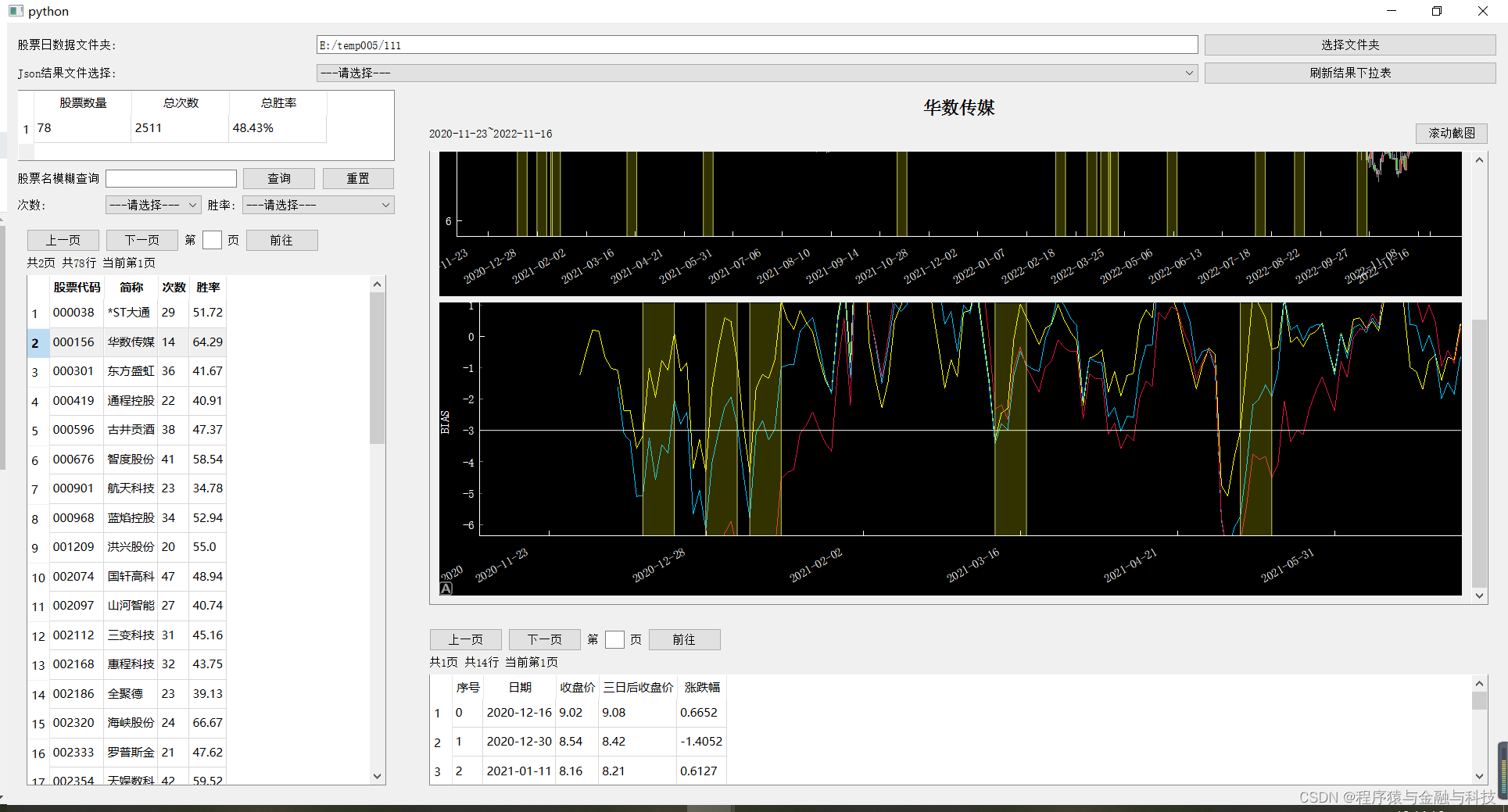
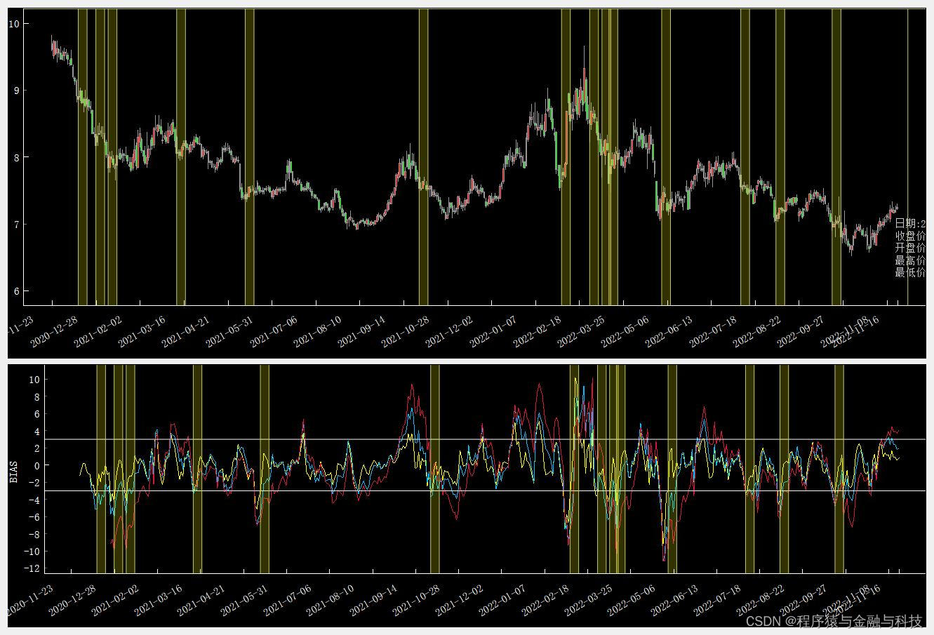
所谓BIAS乖离率,是指股价与移动平均线之间的偏离程度。它是根据移动平均线的原理派生的一项技术指标,通过测算股价在波动过程中与移动平均线出现偏离的程度,从而得出股价在剧烈波动时因偏离移动平均趋势而造成可能的回档或反弹,以及股价在正常波动范围内移动而形成继续原有趋势的可信度。
BIAS乖离率主要应用于预测股价的暴涨或暴跌。当股价在下方远离移动平均线时,投资者可适当地买进;当股价在上方远离移动平均线时,投资者可以考虑卖出。乖离率计算公式具体如下。
乖离率=(当日收盘价-N日内移动平均价)/N日内移动平均价 * 100%
5日乖离率=(当日收盘价-5日内移动平均价)/5日内移动平均价*100%
公式中的N日按照选定的移动平均线日数确定,一般定为5或10。由计算公式可以看出,当股价在移动平均线之上时,称为正乖离率,反之称为负乖离率;当股价与移动平均线重合,乖离率为零。在股价的升降过程中,乖离率反复在零点两侧变化,数值的大小对未来股价的走势分析具有一定的预测功能。正乖离率超过一定数值时,显示短期内多头获利较大,获利回吐的可能性也大,呈卖出信号;负乖离率超过一定数值时,说明空头回补的可能性较大,呈买入信号。
策略代码
本策略BIAS使用与同花顺一样的参数,6日均线,参考上限值3,参考下限值-3
def excute_strategy(base_data,data_dir):
    '''
    指标买点分析技法 - 运用BIAS乖离率指标选择买点
    解析:
    选择买点依据:(本策略使用与同花顺BIAS相同的参数)
    负乖离率从下上穿-3轴,为买入点
    自定义:
    1. 买入时点 =》 走势确定后下一交易日
    2. 胜 =》 买入后第三个交易日收盘价上升,为胜
    只计算最近两年的数据
    :param base_data:股票代码与股票简称 键值对
    :param data_dir:股票日数据文件所在目录
    :return:
    '''
    import pandas as pd
    import numpy as np
    import talib,os
    from datetime import datetime
    from dateutil.relativedelta import relativedelta
    from tools import stock_factor_caculate

    def res_pre_two_year_first_day():
        pre_year_day = (datetime.now() - relativedelta(years=2)).strftime('%Y-%m-%d')
        return pre_year_day
    caculate_start_date_str = res_pre_two_year_first_day()

    dailydata_file_list = os.listdir(data_dir)

    total_count = 0
    total_win = 0
    check_count = 0
    list_list = []
    detail_map = {}
    factor_list = ['BIAS']
    ma_list = []
    for item in dailydata_file_list:
        item_arr = item.split('.')
        ticker = item_arr[0]
        secName = base_data[ticker]
        file_path = data_dir + item
        df = pd.read_csv(file_path,encoding='utf-8')
        # 删除停牌的数据
        df = df.loc[df['openPrice'] > 0].copy()
        df['o_date'] = df['tradeDate']
        df['o_date'] = pd.to_datetime(df['o_date'])
        df = df.loc[df['o_date'] >= caculate_start_date_str].copy()
        # 保存未复权收盘价数据
        df['close'] = df['closePrice']
        # 计算前复权数据
        df['openPrice'] = df['openPrice'] * df['accumAdjFactor']
        df['closePrice'] = df['closePrice'] * df['accumAdjFactor']
        df['highestPrice'] = df['highestPrice'] * df['accumAdjFactor']
        df['lowestPrice'] = df['lowestPrice'] * df['accumAdjFactor']

        if len(df)<=0:
            continue

        # 开始计算
        for item in factor_list:
            df = stock_factor_caculate.caculate_factor(df,item)
        for item in ma_list:
            df = stock_factor_caculate.caculate_factor(df,item)
        df.reset_index(inplace=True)
        df['i_row'] = [i for i in range(len(df))]
        df['three_chg'] = round(((df['close'].shift(-3) - df['close']) / df['close']) * 100, 4)
        df['three_after_close'] = df['close'].shift(-3)

        df['target_yeah'] = 0
        df.loc[(df['bias'].shift(1)<-3) & (df['bias']>=-3),'target_yeah'] = 1

        i_row_list = df.loc[df['target_yeah']==1]['i_row'].values.tolist()

        node_count = 0
        node_win = 0
        duration_list = []
        table_list = []
        for i,row0 in enumerate(i_row_list):
            row = row0 + 1
            if row >= len(df):
                continue
            date_str = df.iloc[row]['tradeDate']
            cur_close = df.iloc[row]['close']
            three_after_close = df.iloc[row]['three_after_close']
            three_chg = df.iloc[row]['three_chg']

            table_list.append([
                i,date_str,cur_close,three_after_close,three_chg
            ])
            duration_list.append([row-2,row+3])
            node_count += 1
            if three_chg<0:
                node_win +=1
            pass

        list_list.append({
            'ticker':ticker,
            'secName':secName,
            'count':node_count,
            'win':0 if node_count<=0 else round((node_win/node_count)*100,2)
        })
        detail_map[ticker] = {
            'table_list': table_list,
            'duration_list': duration_list
        }

        total_count += node_count
        total_win += node_win
        check_count += 1
        pass
    df = pd.DataFrame(list_list)

    results_data = {
        'check_count':check_count,
        'total_count':total_count,
        'total_win':0 if total_count<=0 else round((total_win/total_count)*100,2),
        'start_date_str':caculate_start_date_str,
        'df':df,
        'detail_map':detail_map,
        'factor_list':factor_list,
        'ma_list':ma_list
    }
    return results_data
结果
本文校验的数据是随机抽取的81个股票


 342
342


 被折叠的 条评论
为什么被折叠?
被折叠的 条评论
为什么被折叠?
 到【灌水乐园】发言


