


Anomaly Detection 异常检测
异常数据的检测,这实际上也是一种无监督学习(因为不知道什么是异常)
1.导入
import numpy as np
import matplotlib.pyplot as plt
from utils import *

%matplotlib inline
文件utils.py的代码:
import numpy as np
import matplotlib.pyplot as plt

def load_data():
    X = np.load("data/X_part1.npy")
    X_val = np.load("data/X_val_part1.npy")
    y_val = np.load("data/y_val_part1.npy")
    return X, X_val, y_val

def load_data_multi():
    X = np.load("data/X_part2.npy")
    X_val = np.load("data/X_val_part2.npy")
    y_val = np.load("data/y_val_part2.npy")
    return X, X_val, y_val


def multivariate_gaussian(X, mu, var):
    """
    Computes the probability
    density function of the examples X under the multivariate gaussian
    distribution with parameters mu and var. If var is a matrix, it is
    treated as the covariance matrix. If var is a vector, it is treated
    as the var values of the variances in each dimension (a diagonal
    covariance matrix
    """

    k = len(mu)

    if var.ndim == 1:
        var = np.diag(var)

    X = X - mu
    p = (2* np.pi)**(-k/2) * np.linalg.det(var)**(-0.5) * \
        np.exp(-0.5 * np.sum(np.matmul(X, np.linalg.pinv(var)) * X, axis=1))

    return p

def visualize_fit(X, mu, var):
    """
    This visualization shows you the
    probability density function of the Gaussian distribution. Each example
    has a location (x1, x2) that depends on its feature values.
    """

    X1, X2 = np.meshgrid(np.arange(0, 35.5, 0.5), np.arange(0, 35.5, 0.5))
    Z = multivariate_gaussian(np.stack([X1.ravel(), X2.ravel()], axis=1), mu, var)
    Z = Z.reshape(X1.shape)

    plt.plot(X[:, 0], X[:, 1], 'bx')

    if np.sum(np.isinf(Z)) == 0:
        plt.contour(X1, X2, Z, levels=10**(np.arange(-20., 1, 3)), linewidths=1)

    # Set the title
    plt.title("The Gaussian contours of the distribution fit to the dataset")
    # Set the y-axis label
    plt.ylabel('Throughput (mb/s)')
    # Set the x-axis label
    plt.xlabel('Latency (ms)')
2.Anomaly Detection 异常检测
2.1 问题描述
在本练习中,您将实现异常检测算法以检测服务器计算机中的异常行为。
数据集包含两个特征:
- 吞吐量(mb/s)和
- 每个服务器的响应延迟(ms)。
当您的服务器运行时,您收集了 m = 307 m=307 m=307它们的行为示例,因此有一个未标记的数据集 { x ( 1 ) , … , x ( m ) } \{x^{(1)}, \ldots, x^{(m)}\} {x(1),…,x(m)}.
- 您怀疑这些示例中的绝大多数是服务器正常运行的“正常”(非异常)示例,但也可能有一些服务器在该数据集中异常运行的示例。
您将使用高斯模型来检测您的数据集。
- 您将首先从2D数据集开始,该数据集将允许您可视化算法正在做什么。
- 在该数据集上,您将拟合高斯分布,然后找到概率非常低的值,因此可以认为是异常。
- 之后,您将把异常检测算法应用于具有多个维度的更大数据集。
2.2 数据集
您将从加载此任务的数据集开始。
- 下面显示的
load_data()函数将数据加载到变量X_train、X_val和y_val中 - 您将使用
X_train拟合高斯分布 - 您将使用
X_val和y_val作为交叉验证集来选择阈值并确定异常与正常示例
# Load the dataset
X_train, X_val, y_val = load_data()
查看前五条数据
# Display the first five elements of X_train
print("The first 5 elements of X_train are:\n", X_train[:5])

# Display the first five elements of X_val
print("The first 5 elements of X_val are\n", X_val[:5])

# Display the first five elements of y_val
print("The first 5 elements of y_val are\n", y_val[:5])
检查shape
print ('The shape of X_train is:', X_train.shape)
print ('The shape of X_val is:', X_val.shape)
print ('The shape of y_val is: ', y_val.shape)

The shape of X_train is: (307, 2)
The shape of X_val is: (307, 2)
The shape of y_val is:  (307,)
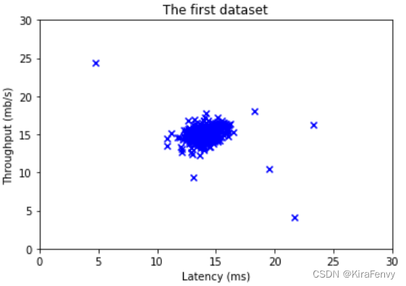
数据可视化:
对于这个数据集,您可以使用散点图来可视化数据(“X_train”),因为它只有两个属性可以绘制(吞吐量和延迟)
# Create a scatter plot of the data. To change the markers to blue "x",
# we used the 'marker' and 'c' parameters
plt.scatter(X_train[:, 0], X_train[:, 1], marker='x', c='b')

# Set the title
plt.title("The first dataset")
# Set the y-axis label
plt.ylabel('Throughput (mb/s)')
# Set the x-axis label
plt.xlabel('Latency (ms)')
# Set axis range
plt.axis([0, 30, 0, 30])
plt.show()
2.3 高斯分布
To perform anomaly detection, you will first need to fit a model to the data’s distribution. 首先要把模型匹配数据分布才能执行异常检测
-
Given a training set { x ( 1 ) , . . . , x ( m ) } \{x^{(1)}, ..., x^{(m)}\} {x(1),...,x(m)} you want to estimate the Gaussian distribution for each of the features x i x_i xi.
-
Recall that the Gaussian distribution is given by
p ( x ; μ , σ 2 ) = 1 2 π σ 2 exp − ( x − μ ) 2 2 σ 2 p(x ; \mu,\sigma ^2) = \frac{1}{\sqrt{2 \pi \sigma ^2}}\exp^{ - \frac{(x - \mu)^2}{2 \sigma ^2} } p(x;μ,σ2)=2πσ21exp−2σ2(x−μ)2
where μ \mu μ is the mean and σ 2 \sigma^2 σ2 controls the variance.
-
For each feature i = 1 … n i = 1\ldots n i=1…n, you need to find parameters μ i \mu_i μi and σ i 2 \sigma_i^2 σi2 that fit the data in the i i i-th dimension { x i ( 1 ) , . . . , x i ( m ) } \{x_i^{(1)}, ..., x_i^{(m)}\} {xi(1),...,xi(m)} (the i i i-th dimension of each example).
2.3.1 Estimating parameters for a Gaussian
Your task is to complete the code in estimate_gaussian below.
Exercise 1
Please complete the estimate_gaussian function below to calculate mu (mean for each feature in X)and var (variance for each feature in X).
You can estimate the parameters, (
μ
i
\mu_i
μi,
σ
i
2
\sigma_i^2
σi2), of the
i
i
i-th
feature by using the following equations. To estimate the mean, you will
use: 平均值的计算公式
μ i = 1 m ∑ j = 1 m x i ( j ) \mu_i = \frac{1}{m} \sum_{j=1}^m x_i^{(j)} μi=m1j=1∑mxi(j)
and for the variance you will use: 方差的计算公式
σ
i
2
=
1
m
∑
j
=
1
m
(
x
i
(
j
)
−
μ
i
)
2
\sigma_i^2 = \frac{1}{m} \sum_{j=1}^m (x_i^{(j)} - \mu_i)^2
σi2=m1j=1∑m(xi(j)−μi)2
# UNQ_C1
# GRADED FUNCTION: estimate_gaussian

def estimate_gaussian(X):
    """
    Calculates mean and variance of all features
    in the dataset

    Args:
        X (ndarray): (m, n) Data matrix

    Returns:
        mu (ndarray): (n,) Mean of all features
        var (ndarray): (n,) Variance of all features
    """

    m, n = X.shape

    ### START CODE HERE ###
    mu = np.mean(X,axis = 0)#别忘了要指定轴
    var = np.mean((X - mu)**2,axis = 0) ##注意**2是在sum里面的
    ### END CODE HERE ###

    return mu, var
函数调用:
# Estimate mean and variance of each feature
mu, var = estimate_gaussian(X_train)

print("Mean of each feature:", mu)
print("Variance of each feature:", var)

Mean of each feature: [14.11222578 14.99771051]
Variance of each feature: [1.83263141 1.70974533]
# Returns the density of the multivariate normal
# at each data point (row) of X_train
p = multivariate_gaussian(X_train, mu, var)

#Plotting code
visualize_fit(X_train, mu, var)
2.3.2 选择阈值
已经估计了高斯参数,您可以研究在给定这种分布的情况下,哪些示例具有非常高的概率,哪些示例的概率非常低。
- 低概率的例子更可能是我们数据集中的异常。
- 确定哪些示例是异常的一种方法是基于交叉验证集选择阈值。
在本节中,您将完成“select_threshold”中的代码,以使用交叉验证集上的 F 1 F_1 F1分数选择阈值 ε \varepsilon ε。
- For this, we will use a cross validation set
{ ( x c v ( 1 ) , y c v ( 1 ) ) , … , ( x c v ( m c v ) , y c v ( m c v ) ) } \{(x_{\rm cv}^{(1)}, y_{\rm cv}^{(1)}),\ldots, (x_{\rm cv}^{(m_{\rm cv})}, y_{\rm cv}^{(m_{\rm cv})})\} {(xcv(1),ycv(1)),…,(xcv(mcv),ycv(mcv))}, where the label y = 1 y=1 y=1 corresponds to an anomalous example, and y = 0 y=0 y=0 corresponds to a normal example. y=1代表异常数据,y=0代表正常数据 - For each cross validation example, we will compute
p
(
x
c
v
(
i
)
)
p(x_{\rm cv}^{(i)})
p(xcv(i)). The vector of all of these probabilities
p
(
x
c
v
(
1
)
)
,
…
,
p
(
x
c
v
(
m
c
v
)
)
p(x_{\rm cv}^{(1)}), \ldots, p(x_{\rm cv}^{(m_{\rm cv)}})
p(xcv(1)),…,p(xcv(mcv)) is passed to
select_thresholdin the vectorp_val. - The corresponding labels
y
c
v
(
1
)
,
…
,
y
c
v
(
m
c
v
)
y_{\rm cv}^{(1)}, \ldots, y_{\rm cv}^{(m_{\rm cv)}}
ycv(1),…,ycv(mcv) is passed to the same function in the vector
y_val.
Exercise 2
Please complete the select_threshold function below to find the best threshold to use for selecting outliers based on the results from a 验证集validation set (p_val) and the ground truth (y_val). 完成下列函数
-
In the provided code
select_threshold, 已经有一个循环将尝试 ε \varepsilon ε的许多不同值,并根据 F 1 F_1 F1得分选择最佳 ε \varepsilon ε。 -
通过选择
epsilon作为阈值来计算F1分数,并将值放在“F1”中。-
Recall that if an example x x x has a low probability p ( x ) < ε p(x) < \varepsilon p(x)<ε, then it is classified as an anomaly. 如果x的概率小于阈值,就是异常数据
-
Then, you can compute precision 准确率(预测当中正确预测概率) and recall 召回率(阳性当中被正确预测概率) by:
p r e c = t p t p + f p r e c = t p t p + f n , \begin{aligned} prec&=&\frac{tp}{tp+fp}\\ rec&=&\frac{tp}{tp+fn}, \end{aligned} precrec==tp+fptptp+fntp, where- t p tp tp is the number of true positives: the ground truth label says it’s an anomaly and our algorithm correctly classified it as an anomaly. 真阳性
- f p fp fp is the number of false positives: the ground truth label says it’s not an anomaly, but our algorithm incorrectly classified it as an anomaly. 假阳性
- f n fn fn is the number of false negatives: the ground truth label says it’s an anomaly, but our algorithm incorrectly classified it as not being anomalous. 假阴性
-
The F 1 F_1 F1 score is computed using precision ( p r e c prec prec) and recall ( r e c rec rec) as follows: 计算F1分数的公式
F 1 = 2 ⋅ p r e c ⋅ r e c p r e c + r e c F_1 = \frac{2\cdot prec \cdot rec}{prec + rec} F1=prec+rec2⋅prec⋅rec
-
Implementation Note:
In order to compute
t
p
tp
tp,
f
p
fp
fp and
f
n
fn
fn, you may be able to use a vectorized implementation rather than loop over all the examples. 使用向量化的实现方式而不是循环
代码填空:
下面代码选择epsilon的方法是把概率最大值和最小值区间内分成一千份,然后遍历
# UNQ_C2
# GRADED FUNCTION: select_threshold

def select_threshold(y_val, p_val):
    """
    Finds the best threshold to use for selecting outliers
    based on the results from a validation set (p_val)
    and the ground truth (y_val)

    Args:
        y_val (ndarray): Ground truth on validation set
        p_val (ndarray): Results on validation set

    Returns:
        epsilon (float): Threshold chosen
        F1 (float):      F1 score by choosing epsilon as threshold
    """

    best_epsilon = 0
    best_F1 = 0
    F1 = 0

    step_size = (max(p_val) - min(p_val)) / 1000

    for epsilon in np.arange(min(p_val), max(p_val), step_size):

        ### START CODE HERE ###
        predictions = # Your code here to calculate predictions for each example using epsilon as threshold

        tp = # Your code here to calculate number of true positives
        fp = # Your code here to calculate number of false positives
        fn = # Your code here to calculate number of false negatives

        prec = # Your code here to calculate precision
        rec = # Your code here to calculate recall

        F1 = # Your code here to calculate F1
        ### END CODE HERE ###

        if F1 > best_F1:
            best_F1 = F1
            best_epsilon = epsilon

    return best_epsilon, best_F1
答案:
    for epsilon in np.arange(min(p_val), max(p_val), step_size):
        ### START CODE HERE ###
        predictions = (p_val < epsilon)

        tp = np.sum((predictions == 1) & (y_val == 1))
        fp = np.sum((predictions == 1) & (y_val == 0))# Your code here to calculate number of false positives
        fn = np.sum((predictions == 0) & (y_val == 1))# Your code here to calculate number of false negatives

        prec = tp / (tp + fp)
        rec = tp / (tp + fn)

        F1 = 2 * prec * rec / (prec + rec)# Your code here to calculate F1
        ### END CODE HERE ###

        if F1 > best_F1:
            best_F1 = F1
            best_epsilon = epsilon

    return best_epsilon, best_F1
测试代码:
p_val = multivariate_gaussian(X_val, mu, var)
epsilon, F1 = select_threshold(y_val, p_val)

print('Best epsilon found using cross-validation: %e' % epsilon)
print('Best F1 on Cross Validation Set: %f' % F1)

Best epsilon found using cross-validation: 8.990853e-05
Best F1 on Cross Validation Set: 0.875000
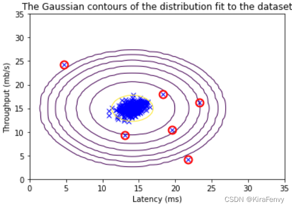
可视化异常数据
# Find the outliers in the training set
outliers = p < epsilon

# Visualize the fit
visualize_fit(X_train, mu, var)

# Draw a red circle around those outliers
plt.plot(X_train[outliers, 0], X_train[outliers, 1], 'ro',
         markersize= 10,markerfacecolor='none', markeredgewidth=2)
2.4 在大数据集上的实践
In this dataset, each example is described by 11 features, capturing many more properties of your compute servers.
- The
load_data()function shown below loads the data into variablesX_train_high,X_val_highandy_val_high_highis meant to distinguish these variables from the ones used in the previous part- We will use
X_train_highto fit Gaussian distribution - We will use
X_val_highandy_val_highas a cross validation set to select a threshold and determine anomalous vs normal examples
- 下面显示的“load_data()”函数将数据加载到变量“X_train_high”、“X_val_high”和“y_val_high”中`
- “_high”意在将这些变量与前一部分中使用的变量区分开来
- 我们将使用“X_train_high”来拟合高斯分布
- 我们将使用“X_val_high”和“y_val_high”作为交叉验证集来选择阈值并确定异常与正常示例
加载数据
# load the dataset
X_train_high, X_val_high, y_val_high = load_data_multi()
查看数据维度
print ('The shape of X_train_high is:', X_train_high.shape)
print ('The shape of X_val_high is:', X_val_high.shape)
print ('The shape of y_val_high is: ', y_val_high.shape)
进行异常检测
The code below will use your code to
- Estimate the Gaussian parameters ( μ i \mu_i μi and σ i 2 \sigma_i^2 σi2)
- Evaluate the probabilities for both the training data
X_train_highfrom which you estimated the Gaussian parameters, as well as for the the cross-validation setX_val_high. 评估用于估计高斯参数的训练数据“X_train_high”以及交叉验证集“X_val_high”的概率。 - Finally, it will use
select_thresholdto find the best threshold ε \varepsilon ε.
# Apply the same steps to the larger dataset

# Estimate the Gaussian parameters
mu_high, var_high = estimate_gaussian(X_train_high)

# Evaluate the probabilites for the training set
p_high = multivariate_gaussian(X_train_high, mu_high, var_high)

# Evaluate the probabilites for the cross validation set
p_val_high = multivariate_gaussian(X_val_high, mu_high, var_high)

# Find the best threshold
epsilon_high, F1_high = select_threshold(y_val_high, p_val_high)

print('Best epsilon found using cross-validation: %e'% epsilon_high)
print('Best F1 on Cross Validation Set:  %f'% F1_high)
print('# Anomalies found: %d'% sum(p_high < epsilon_high))


Best epsilon found using cross-validation: 1.377229e-18
Best F1 on Cross Validation Set:  0.615385
# Anomalies found: 117
3.课后题
- 监督学习和异常检测的使用:
- 您正在构建一个系统来检测数据中心中的计算机是否出现故障。您有10000个数据点计算机运行良好,并且没有来自计算机的数据发生故障。使用异常检测
- 您正在构建一个系统来检测数据中心中的计算机是否出现故障。你有10000个数据点计算机运行良好,10000个计算机数据点出现故障。使用监督学习
- 上面的使用场景很容易判断,但要是有已知异常数据但极少要怎么办?
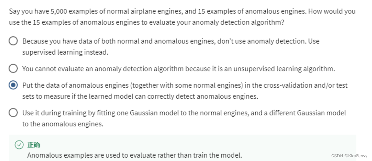
将异常发动机的数据(与一些正常发动机一起)进行交叉验证和/或测试
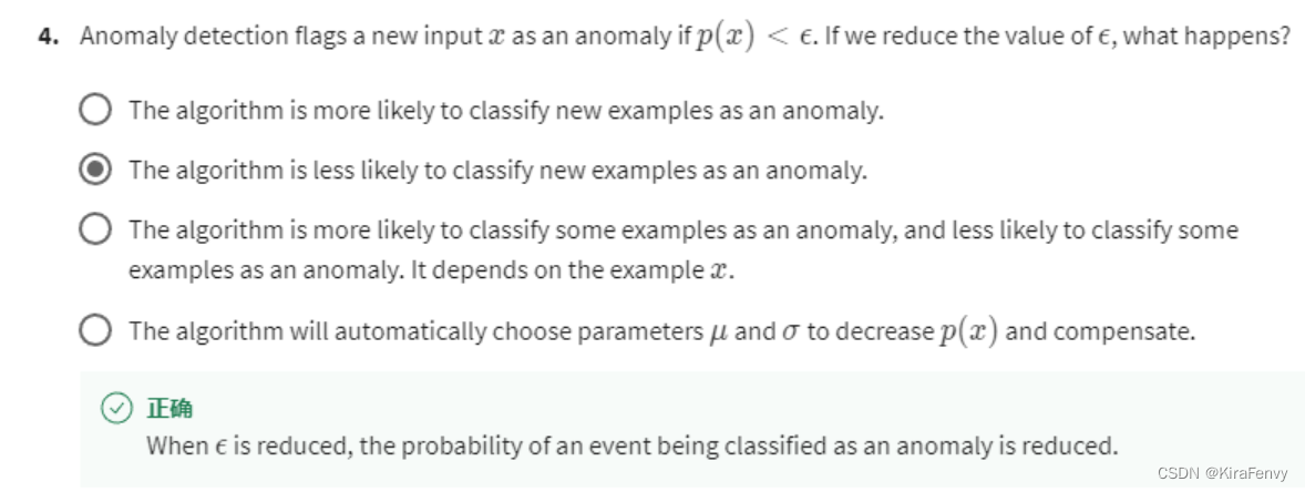
-
阈值变小了,更少的数据会被分配为异常数据
-
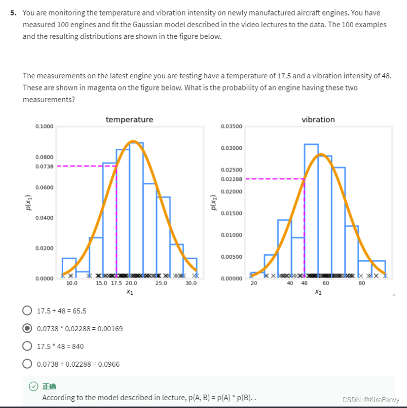
你正在监测新制造的飞机发动机的温度和振动强度。测量了100个引擎,并将视频讲座中描述的高斯模型与数据拟合。100个示例所得分布如下图所示。
您正在测试的最新发动机的测量值温度为17.5,振动强度为48。下图中以洋红色表示。发动机有这两种情况的概率是多少


 1932
1932


 被折叠的 条评论
为什么被折叠?
被折叠的 条评论
为什么被折叠?
 到【灌水乐园】发言


