


附上资源链接:pytorch实现天气分类-深度学习文档类资源-CSDN文库
1.总体流程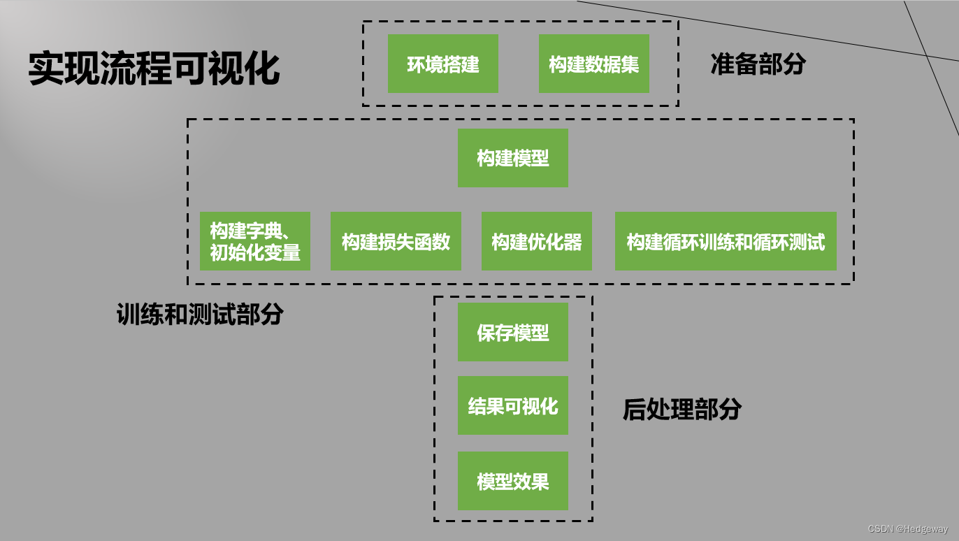
2.代码
①数据集划分
import splitfolders

splitfolders.ratio(input='dataset', output='output', ratio=(0.8, 0.2))
②全部流程
import torch
import torch.nn as nn
import matplotlib.pyplot as plt # 用来画准确度和损失值
import torch.nn.functional as F # 导入relu归一化函数,该模块包含torch.nn库中的所有函数(而该库的其他部分包含类,即上面)
import torchvision # 用来导入数据集
import os
from torchvision import transforms
from torch.utils.data import TensorDataset
from tqdm import tqdm # 进度条
# 数据处理
# 将所有变换都以列表形式放在Compose里面
transform = transforms.Compose([
# 将图片切割为96*96的大小
transforms.Resize((128, 128)),
# 依据概率p对图片进行垂直翻转
# torchvision.transforms.RandomHorizontalFlip(p=0.3),
# 将读取的图片或者其他类型的数据转换成张量
transforms.ToTensor(),
# 将图片进行归一化处理
transforms.Normalize(mean=[0.5, 0.5, 0.5], std=[0.5, 0.5, 0.5])
])
# 数据集路径
baseDir = 'E:\\xiaoA_suanfa\\three_and_final\\final\\output'
# baseDir里面包含训练集和测试集两个文件夹
trainDir = os.path.join(baseDir, 'train')
testDir = os.path.join(baseDir, 'test')
trainSet = torchvision.datasets.ImageFolder(trainDir, transform=transform)
testSet = torchvision.datasets.ImageFolder(testDir, transform=transform)
# torch.utils.data.DataLoader数据加载器,结合了数据集和取样器,并且可以提供多个线程处理数据集。
# 在训练模型时使用到此函数,用来把训练数据分成多个小组,此函数每次抛出一组数据。
# 直至把所有的数据都抛出。
BATCH_SIZE = 30 # 每一批的图片数量为30
trainLoader = torch.utils.data.DataLoader(trainSet, batch_size=BATCH_SIZE, shuffle=True)
testLoader = torch.utils.data.DataLoader(testSet, batch_size=BATCH_SIZE,)
"""-------------------------------------------------------------------------------------"""
# 迭代器,作用与enumerate差不多
imgs, labels = next(iter(trainLoader))
# 交换类别和索引的位置,便于后面训练
id_to_class = dict((v, k) for k, v in trainSet.class_to_idx.items())
"""
# 画出数据集中的一些图片
plt.figure(figsize=(12, 8)) # 整张画布的横长和纵长
for i, (img, label) in enumerate(zip(imgs[:9], labels[:9])):
img = (img.permute(1, 2, 0) + 1) / 2 # 对三通道图片进行处理,才能plt.imshow()出来
# 比如图片img的size比如是(3,96,96)就可以利用img.permute(1,2,0)
# 得到一个size为(96,96,3)的tensor,和view()差不多
plt.subplot(3, 3, i+1) # 三行三列第i+1个子图,i从0开始
plt.title(id_to_class.get(label.item())) # 标题打上类别
plt.imshow(img)"""
"""******************************************************************************"""
# 构建一个简单的神经网络:三层卷积池化+三层全连接层
# bn层,softout,dropout层
class Net(nn.Module):
def __init__(self):
super(Net, self).__init__()
# 卷积核的作用是提取特征,因为特征相邻相似
# 三通道,16个卷积核,尺寸为3*3*3 # 96 * 96像素 > 94 * 94 : poolm1 : 47 * 47
#256,254,127
#128,126,63
self.conv1 = nn.Conv2d(in_channels=3, out_channels=16, kernel_size=3)
# 47 * 47 > 45 * 45 : poolm2 : 22 * 22
#127,125,62
#63,61,30
self.conv2 = nn.Conv2d(in_channels=16, out_channels=32, kernel_size=3)
# 22 * 22 > 20 *20 : poolm1 : 10 * 10
# 62,60,30
#30,28,14
self.conv3 = nn.Conv2d(in_channels=32, out_channels=64, kernel_size=3)
# 池化核的作用是降维、去除冗余信息、对特征进行压缩、
# 简化网络复杂度、减小计算量、减小内存消耗等,从而提高运算速度,降低过拟合。
self.poolm1 = nn.MaxPool2d(kernel_size=2, stride=2)
self.poolm2 = nn.MaxPool2d(kernel_size=3, stride=2)
# 10 * 10特征图尺寸, 64是通道数, 给1024个神经元
self.fc1 = nn.Linear(14*14 * 64, 1024)
# 1024个神经元给512个神经元
self.fc2 = nn.Linear(1024, 512)
# 512个神经元给11个类别, 一定要跟类别数相同,这里不softmax的原因是后面交叉熵函数有softmax+nllloss
self.fc3 = nn.Linear(512, 11)
def forward(self, x):
# relu是激活函数:为了增加神经网络模型的非线性;
# softmax是归一化函数,交叉熵函数(指标)包括softmax归一化函数和损失函数nllloss
x = F.relu(self.conv1(x))
x = self.poolm1(x)
x = F.relu(self.conv2(x))
x = self.poolm2(x)
x = F.relu(self.conv3(x))
x = self.poolm1(x)
x = x.view(-1, 14*14 * 64)
x = F.relu(self.fc1(x))
x = F.relu(self.fc2(x))
x = self.fc3(x)
return x # 返回11类的概率,后面交叉熵函数再进行归一化
# bn层,softout,dropout层
# 1.神经网络各个层的作用,如何计算尺寸和与batchsize、dataloader区分
# 2.Imageloader的作用是按照文件夹格式读取照片,dataloader是具有迭代功能数据加载器,
# 每次从imageloader里面随机抓取bacth_size张图片
# 3.显示图片时plt是pycharm显示的,PIL直接本地查看器
# 4.tqdm进度条,直接把dataloader给tqdm,显示总共的批次数;enumerate对批次数进行循环
model = Net() # 创建实例
print(model)
# 是否利用GPU进行加速
device = "cuda:0" if torch.cuda.is_available() else "cpu"
model.to(device)
# 交叉熵损失函数:softmax归一化和nllloss损失函数
criterion = nn.CrossEntropyLoss()
# 梯度下降优化器
optimizer = torch.optim.Adam(model.parameters())
# 创建字典用来存储训练损失值和准确值
trainhistory = {'Train Loss': [], 'Train Accuracy': []}
# 创建字典用来存储测试损失值和准确值
testhistory = {'Test Loss': [], 'Test Accuracy': []}
# 训练次数
epochs = 12
# 开始训练
for epoch in range(epochs):
trcorrect = 0 # 训练时识别正确个数
trtotal = 0 # 标签个数
totaltrloss = 0 # 训练时总损失值
tr_epoch_loss = 0 # 训练损失值
tr_epoch_acc = 0 # 训练准确度
epoch_test_loss = 0 # 测试损失值
epoch_test_acc = 0 # 测试准确度
testAccuracy = 0 # 测试准确度
testLoss = 0 # 测试损失值
processBar = tqdm(trainLoader, unit='batch_idx') # 构建进度条
model.train(True) # 开始训练
for batch_idx, (trainimgs, trlabels) in enumerate(processBar):
trainimgs = trainimgs.to(device) # 是否使用GPU
trlabels = trlabels.to(device) # 是否使用GPU
optimizer.zero_grad() # 将梯度置零
outputs = model(trainimgs) # 传入一批数据进行训练
trloss = criterion(outputs, trlabels) # 计算此次循环的训练误差
trpredictions = torch.argmax(outputs, dim=1) # 得出本次训练的结果
accuracy = torch.sum(trpredictions == trlabels) / labels.shape[0] # 进行比较,加和,相除,得出每次训练循环的准确度
trcorrect += (trpredictions == trlabels).sum().item() # 总训练准确度,后面还要除以总数量
trtotal += trlabels.size(0)
totaltrloss += trloss.item() # 总训练误差,后面还要除以总数量
trloss.backward() # 反向传播,计算权重weight和偏置bias,将反向传播的梯度信息传给下面的优化器
optimizer.step() # 更新权重weight和偏置bias
# 更新进度条
processBar.set_description("[%d/%d] Loss: %.4f, Acc: %.4f" %
(epoch+1, epochs, trloss.item(), accuracy.item()))
# 一个大循环内,当训练集到最后一批数据时,进行测试,意味着最后这一小批训练数据没有进行训练,可能导致准确度下降,问题不大
if batch_idx == len(processBar) - 1:
correct, totaltestLoss = 0, 0
model.train(False) # 关闭训练
with torch.no_grad(): # 此时没有训练,所以省去梯度,节省内存开销
for testimgs,testlabels in testLoader: # 对测试集的每一批数据进行测试
testimgs = testimgs.to(device) # 是否使用GPU
testlabels = testlabels.to(device) # 是否使用GPU
testoutputs = model(testimgs) # 把图片传入到模型中,利用训练好的参数进行测试
loss = criterion(testoutputs, testlabels) # 计算损失值
testpredictions = torch.argmax(testoutputs, dim=1) # 得出最大概率,得出预测分类
totaltestLoss += loss # 总测试误差
correct += torch.sum(testpredictions == testlabels) # 正确预测总个数
testLoss = totaltestLoss / len(testLoader) # 测试误差
testAccuracy = correct / (BATCH_SIZE * len(testLoader)) # 测试准确度
# 进度条显示
processBar.set_description("[%d/%d] Train Loss: %.4f, Train Acc: %.4f; "
"Test Loss: %.4f, Test Acc: %.4f" %
(epoch + 1, epochs, trloss, accuracy, testLoss, testAccuracy))
testhistory['Test Accuracy'].append(testAccuracy.cpu()) # 添加到测试准确度字典里面
testhistory['Test Loss'].append(testLoss.cpu()) # 添加到测试误差字典里面
tr_epoch_loss = totaltrloss / len(trainLoader) # 本次训练误差
tr_epoch_acc = trcorrect / trtotal # 本次训练准确度
trainhistory['Train Accuracy'].append(tr_epoch_acc) # 添加到训练准确度字典里面
trainhistory['Train Loss'].append(tr_epoch_loss) # 添加到训练误差字典里面
# 二行二列第一幅图画训练误差
plt.subplot(2,2,1)
plt.plot(trainhistory['Train Loss'], color='blue', label='Train Loss')
plt.legend(loc='best') # 将图标置于最好位置
plt.grid(True) # 开启网格线
plt.xlabel('epochs')
plt.ylabel('trainLoss')
# 二行二列第一幅图画训练准确度
plt.subplot(2, 2, 2)
plt.plot(trainhistory['Train Accuracy'], color='violet', label='Train Accuracy')
plt.legend(loc='best') # 将图标置于最好位置
plt.grid(True) # 开启网格线
plt.xlabel('epochs')
plt.ylabel('trainAccuracy')
# 二行二列第一幅图画测试误差
plt.subplot(2, 2, 3)
plt.plot(testhistory['Test Loss'], color='red', label='Test Loss')
plt.legend(loc='best') # 将图标置于最好位置
plt.grid(True) # 开启网格线
plt.xlabel('epochs')
plt.ylabel('testLoss')
# 二行二列第一幅图画测试准确度
plt.subplot(2, 2, 4)
plt.plot(testhistory['Test Accuracy'], color='green', label='Test Accuracy')
plt.legend(loc='best') # 将图标置于最好位置
plt.grid(True) # 开启网格线
plt.xlabel('epochs')
plt.ylabel('testAccuracy')
plt.show()
# 保存模型
torch.save(model.cpu().state_dict(), './modeldict.pth') # 只保留参数
torch.save(model, './model.pth') # 保留整个模型
"""-----------------------------------------------"""
# 关闭训练
model.train(False)
# 这个顺序很重要,要和训练时候的类名顺序一致
class_names = ['dew', 'fogsmog', 'frost', 'glaze', 'hail', 'lightning',
'rain', 'rainbow', 'rime', 'sandstorm', 'snow']
# 载入模型并读取权重
model.load_state_dict(torch.load('./modeldict.pth'))
model.to(device)
model.eval() # 测试模式
# 图片地址列表
img_paths = ['weatherclasstest\\rain2.jpg', 'weatherclasstest\\rainbow2.jpg', 'weatherclasstest\\snow1.jpg',
'weatherclasstest\\snow3.jpg', 'weatherclasstest\\dew.jpg', 'weatherclasstest\\fogsmog.jpg',
'weatherclasstest\\frost.jpg']
# 对图片地址列表中的每个地址
for path in img_paths:
img = plt.imread(path) # 显示图片的第一种方法
plt.axis('off')
plt.imshow(img)
plt.show()
img = Image.open(path) # 输入地址打开图片
# img.show() # 显示图片的第二种方法
# 拓张维度:
# torch.nn只支持小批次的数据输入,不支持输入单个样本。比如nn.Conv2d接收4D
# tensor作为输入:nSamples * nChannels * Height * Width,
# 如果只有一个样本,那么使用input.unsqueeze(0)来增加一个批次维度。
img_ = transform(img).unsqueeze(0)
img_ = img_.to(device) # 是否使用GPU
outputs = model(img_) # 得出11类概率
_, indice = torch.max(outputs, 1) # 输出概率最大的类别索引,前面是概率值,后面是索引
result = class_names[indice] # 得到类别名称
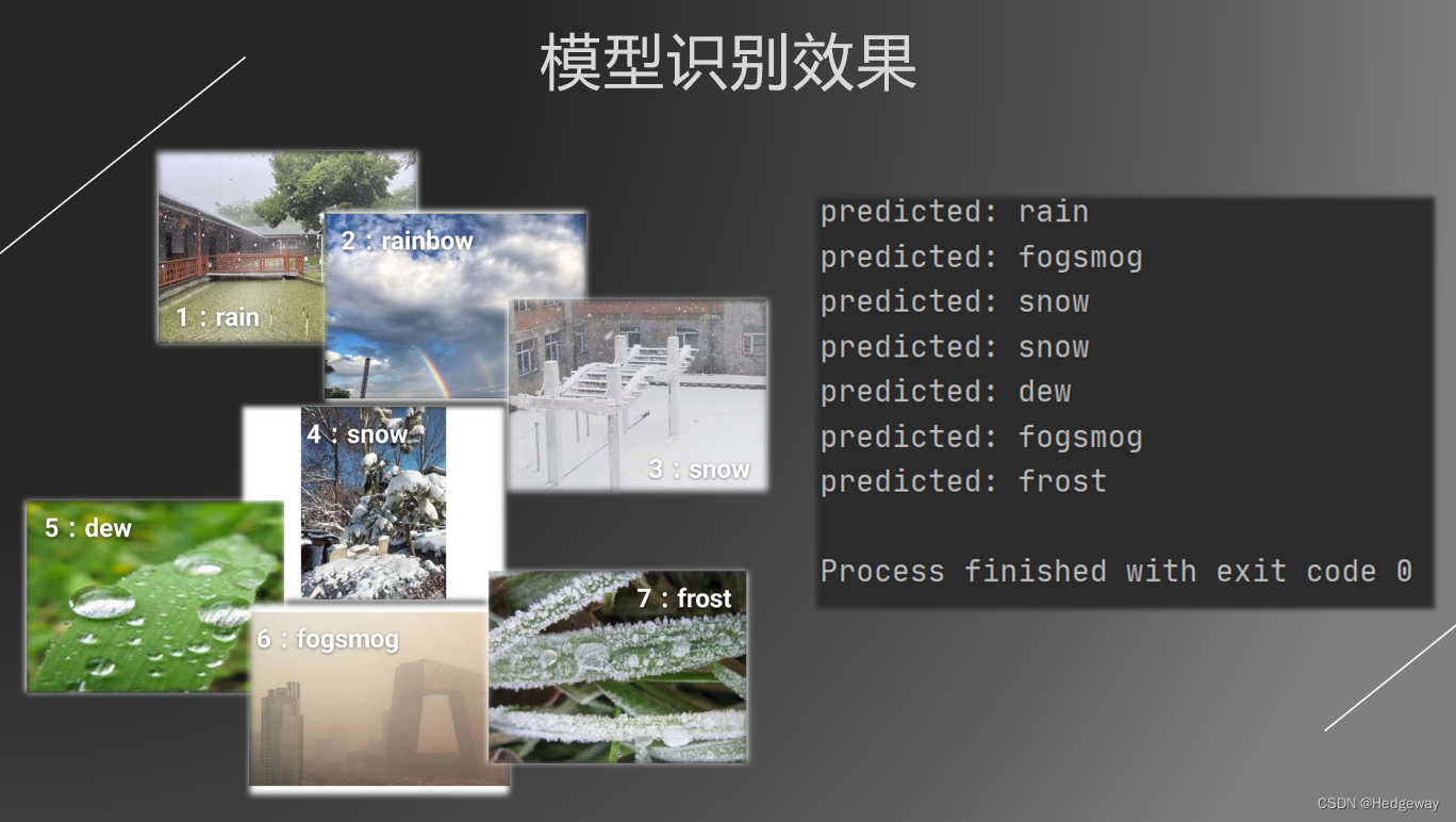
print('predicted:', result) # 输出类别名称
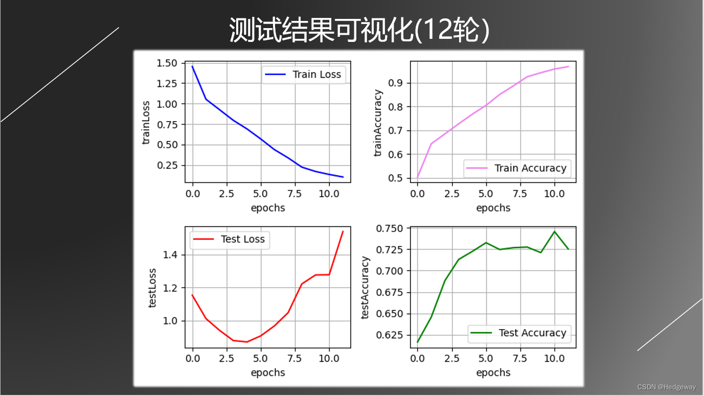
3.过程可视化,测试结果,模型效果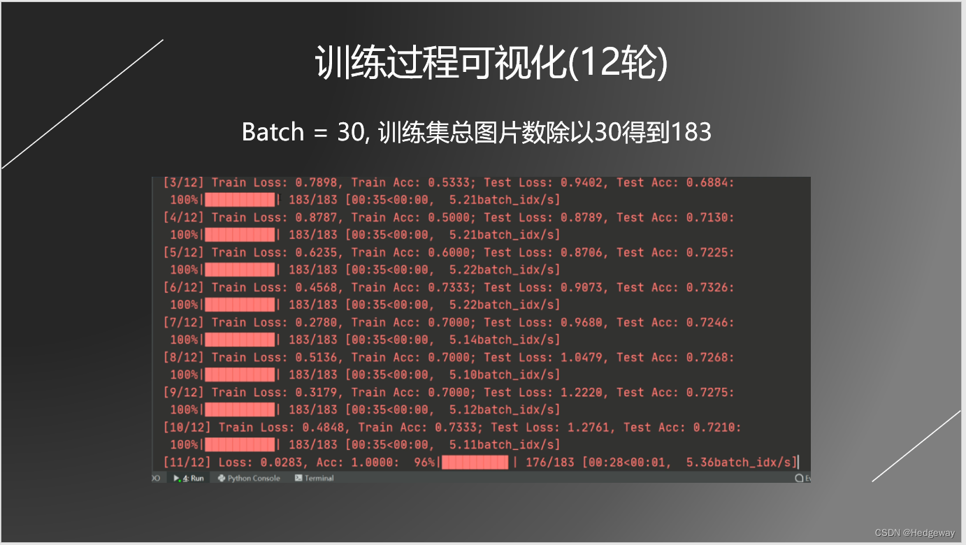


 2272
2272


 被折叠的 条评论
为什么被折叠?
被折叠的 条评论
为什么被折叠?
 到【灌水乐园】发言


