


3. K-Nearest Neighbor
Nearest Neighbor(1NN)
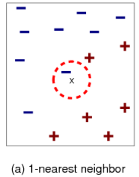
-
To classify a new example x x x:
- Label x x x with the label of the closest example to x x xin the training set.
-
Euclidean Distance
D ( x i , x j ) = ∑ k = 1 d ( x i k − x j k ) 2 D\left(\boldsymbol{x}_i, \boldsymbol{x}_j\right)=\sqrt{\sum\limits_{k=1}^d\left(x_{i k}-x_{j k}\right)^2} D(xi,xj)=k=1∑d(xik−xjk)2
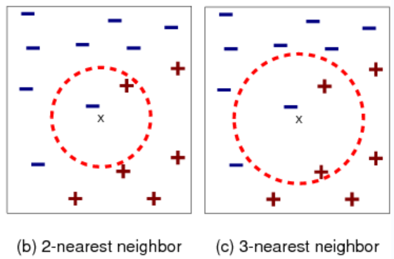
K-Nearest-Neighbors (KNN)
-
Low latitude large-scale data
-
x x x is close to a blue point.
But most of the next closest points are red.
-
Find k k k nearest neighbors of x x x.
-
Label x x x with the majority label within the k k k nearest neighbors
Consider:How can we handle ties for even values of k?
KNN rule is certainly simple and intuitive,but does it work?
KNN is a Goo Approximator on any smooth distribution:
Converges to perfect solution if clear separation
lim n → ∞ ϵ K N N ( n ) ≤ 2 ϵ ∗ ( 1 − ϵ ∗ ) \lim _{n \rightarrow \infty} \epsilon_{\mathrm{KNN}}(n) \leq 2 \epsilon^*\left(1-\epsilon^*\right) n→∞limϵKNN(n)≤2ϵ∗(1−ϵ∗)
(Cover Hart,1969)
KNN is Good Model on complex distributions.
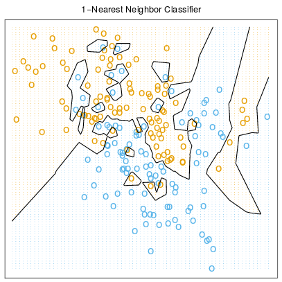
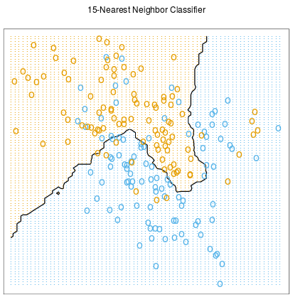
The Effect of K
-
Increasing k simplifies the decision boundary
Majority voting means less emphasis on individual points
-
Choose best k on the validation set.(Often set k as an odd number).
KNN: Inductive Bias
- Similar points have similar labels.
- All dimensions are created equal!
Feature Normalization
- Z-score normalization:
- For each feature dimension j,compute based on its samples:
- Mean μ j = 1 N ∑ i = 1 N x i j \mu_j=\dfrac{1}{N} \sum\limits_{i=1}^N x_{i j} μj=N1i=1∑Nxij
- Variance σ j = 1 N ∑ i = 1 N ( x i j − μ j ) 2 \sigma_j=\sqrt{\dfrac{1}{N} \sum\limits_{i=1}^N\left(x_{i j}-\mu_j\right)^2} σj=N1i=1∑N(xij−μj)2
- Normalize the feature into a new one: x ^ i j ← x i j − μ j σ j \hat{x}_{i j} \leftarrow \dfrac{x_{i j}-\mu_j}{\sigma_j} x^ij←σjxij−μj
Distance Selection
- Cosine Distance: cos ( x i , x j ) = ⟨ x i , x j ⟩ ∥ x i ∥ ∥ x j ∥ \cos \left(\boldsymbol{x_i}, \boldsymbol{x_j}\right)=\dfrac{\left\langle \boldsymbol{x_i}, \boldsymbol{x_j}\right\rangle}{\left\|\boldsymbol{x_i}\right\|\left\|\boldsymbol{x_j}\right\|} cos(xi,xj)=∥xi∥∥xj∥⟨xi,xj⟩
- Minkowski Distance: D p ( x i , x j ) = ∑ k = 1 d ∣ x i k − x j k ∣ p p D_p\left(\boldsymbol{x}_i, \boldsymbol{x}_j\right)=\sqrt[p]{\sum\limits_{k=1}^d\left|x_{i k}-x_{j k}\right|^p} Dp(xi,xj)=pk=1∑d∣xik−xjk∣p
- Mahalanobis Distance: D M ( x i , x j ) = ( x i − x j ) T M ( x i − x j ) D_M\left(\boldsymbol{x}_i, \boldsymbol{x}_j\right)=\sqrt{\left(\boldsymbol{x}_i-\boldsymbol{x}_j\right)^{\mathrm{T}} \boldsymbol{M}\left(\boldsymbol{x}_i-\boldsymbol{x}_j\right)} DM(xi,xj)=(xi−xj)TM(xi−xj)
Weighted KNN
-
Vanilla KNN uses majority vote to predict discrete outputs.
-
Weighted KNN assigns greater weights to closer neighbors.
- Weighting is a common approach used in machine learning.
-
Distance-weighted Classification:
y ^ = argmax c ∈ y ∑ x ′ ∈ KNN c ( x ) 1 D ( x , x ′ ) 2 \hat{y}=\operatorname{argmax}_{c \in y} \sum_{\boldsymbol{x}^{\prime} \in \operatorname{KNN}_c(\boldsymbol{x})} \frac{1}{D\left(\boldsymbol{x}, \boldsymbol{x}^{\prime}\right)^2} y^=argmaxc∈yx′∈KNNc(x)∑D(x,x′)21
-
Distance-weighted Regression:
y ^ = ∑ x ′ ∈ KNN ( x ) 1 D ( x , x ′ ) 2 y ′ \hat{y}=\sum_{x^{\prime} \in \operatorname{KNN}(x)} \frac{1}{D\left(x, x^{\prime}\right)^2} y^{\prime} y^=x′∈KNN(x)∑D(x,x′)21y′
-
Other weighting function (e.g.exponential family)can also be used.
KNN Summary
- When to use:
- Few attributes per instance (expensive computation)
- Lots of training data (curse of dimensionality
- Advantages:
- Agnostically learn complex target functions
- Do not lose information (store original data)
- Data number can be very large (big pro!)
- Class number can be very large (biggest pro!)
- All other ML algorithms may fail here!
- Disadvantages:
- Slow at inference time (acceleration a must)
- Ineffective in high dimensions(curse of dimensionality)
- Fooled easily by irrelevant attributes (feature engineering crucial)


 870
870


 被折叠的 条评论
为什么被折叠?
被折叠的 条评论
为什么被折叠?
 到【灌水乐园】发言


