


秋招面试专栏推荐 :深度学习算法工程师面试问题总结【百面算法工程师】——点击即可跳转
💡💡💡本专栏所有程序均经过测试,可成功执行💡💡💡
专栏目录: 《YOLOv5入门 + 改进涨点》专栏介绍 & 专栏目录 |目前已有50+篇内容,内含各种Head检测头、损失函数Loss、Backbone、Neck、NMS等创新点改进
目前虽然复杂网络的性能很好,但它们日益增加的复杂性给部署带来了挑战。例如,ResNets中的shortcut操作在合并不同层的特征时耗费了大量的off-chip memory traffic。再比如AS-MLP中的axial shift操作以及Swin Transformer中的shift window self-attention操作都需要复杂的工程实现,包括重写CUDA代码。本文介绍的VanillaNet,一种新的神经网络架构,有着简单而优雅的设计,同时在视觉任务中保持了显著的性能。VanillaNet通过舍弃过多的深度、shortcut以及self-attention等复杂的操作,解决了复杂度的问题,非常适合资源有限的环境。文章在介绍主要的原理后,将手把手教学如何进行模块的代码添加和修改,并将修改后的完整代码放在文章的最后,方便大家一键运行,小白也可轻松上手实践。以帮助您更好地学习深度学习目标检测YOLO系列的挑战。
目录
1. 原理

论文地址:VanillaNet: the Power of Minimalism in Deep Learning——点击即可跳转
官方代码: 官方代码仓库——点击即可跳转
VanillaNet:主要原则
VanillaNet 是一种神经网络架构,其设计非常注重简单性和极简主义。以下是对其核心原则和设计理念的详细解释,不包括实验细节:
动机和理念
-
简单胜过复杂:传统的深度学习模型变得越来越复杂,具有复杂的操作层和深度架构。VanillaNet 旨在通过避免过度深度、捷径和自我注意等复杂操作来简化这一点。
-
极简主义设计:该架构采用极简主义,专注于紧凑而直接的层,使其更适合在资源受限的环境中部署。
主要架构特征
-
层结构:VanillaNet 由非常有限数量的卷积层组成。例如,VanillaNet-6 只有六个卷积层。
-
阶段设计:网络分为多个阶段,其中输入特征的大小被下采样,通道数量加倍。这种设计灵感来自 AlexNet 和 VGGNet 等经典神经网络。
-
无捷径:与 ResNet 等架构不同,VanillaNet 不使用捷径连接,从而简化了设计并减少了内存消耗。
-
非线性激活函数:最初,VanillaNet 层包括非线性激活函数,这些函数在训练后会被修剪以返回到更简单的线性形式。
训练技术
-
深度训练策略:VanillaNet 采用独特的训练策略,从包含激活函数的更深层开始,随着训练的进行,这些激活函数逐渐减少为恒等映射。这使得卷积层更容易合并并保持推理速度。
-
基于序列的激活函数:为了增强非线性,VanillaNet 使用基于序列的激活函数,该函数结合了多个可学习的仿射变换。这种方法显著提高了网络的非线性能力,而不会增加复杂性。
性能和效率
-
紧凑高效:尽管 VanillaNet 采用了极简主义方法,但其性能却可与 ResNet 和 Vision Transformers (ViT) 等更复杂的网络相媲美。它证明了简单也可以很强大,为神经网络设计提供了新的视角。
-
资源优化:精简的架构使 VanillaNet 特别适合计算资源有限的环境,例如移动设备和嵌入式系统。
架构细节
-
主干块:初始层使用具有步幅的卷积层将输入图像通道(例如 RGB)转换为更多通道。
-
池化层:最大池化层用于对特征图进行下采样,同时在各个阶段增加通道数量。
-
最终层:网络以平均池化层结束,然后是用于分类任务的完全连接层。
总结
VanillaNet 重新思考了深度学习模型的设计,将架构精简为基本组件,同时仍能实现高性能。它强调极简主义,结合创新的训练技术,展示了深度学习中更简单但有效的模型的潜力。
2. 将VanillaNet添加到yolov5网络中
2.1 VanillaNet代码实现
关键步骤一: 将下面代码粘贴到/projects/yolov5-6.1/models/common.py文件中
class activation(nn.ReLU):
    def __init__(self, dim, act_num=3, deploy=False):
        super(activation, self).__init__()
        self.act_num = act_num
        self.deploy = deploy
        self.dim = dim
        self.weight = torch.nn.Parameter(torch.randn(dim, 1, act_num * 2 + 1, act_num * 2 + 1))
        if deploy:
            self.bias = torch.nn.Parameter(torch.zeros(dim))
        else:
            self.bias = None
            self.bn = nn.BatchNorm2d(dim, eps=1e-6)
        nn.init.trunc_normal_(self.weight, std=.02)

    def forward(self, x):
        if self.deploy:
            return torch.nn.functional.conv2d(
                super(activation, self).forward(x),
                self.weight, self.bias, padding=self.act_num, groups=self.dim)
        else:
            return self.bn(torch.nn.functional.conv2d(
                super(activation, self).forward(x),
                self.weight, padding=self.act_num, groups=self.dim))

    def _fuse_bn_tensor(self, weight, bn):
        kernel = weight
        running_mean = bn.running_mean
        running_var = bn.running_var
        gamma = bn.weight
        beta = bn.bias
        eps = bn.eps
        std = (running_var + eps).sqrt()
        t = (gamma / std).reshape(-1, 1, 1, 1)
        return kernel * t, beta + (0 - running_mean) * gamma / std

    def switch_to_deploy(self):
        kernel, bias = self._fuse_bn_tensor(self.weight, self.bn)
        self.weight.data = kernel
        self.bias = torch.nn.Parameter(torch.zeros(self.dim))
        self.bias.data = bias
        self.__delattr__('bn')
        self.deploy = True


class VanillaStem(nn.Module):
    def __init__(self, in_chans=3, dims=96,
                 k=0, s=0, p=None, g=0, act_num=3, deploy=False, ada_pool=None, **kwargs):
        super().__init__()
        self.deploy = deploy
        stride, padding = (4, 0) if not ada_pool else (3, 1)
        if self.deploy:
            self.stem = nn.Sequential(
                nn.Conv2d(in_chans, dims, kernel_size=k, stride=stride, padding=padding),
                activation(dims, act_num, deploy=self.deploy)
            )
        else:
            self.stem1 = nn.Sequential(
                nn.Conv2d(in_chans, dims, kernel_size=k, stride=stride, padding=padding),
                nn.BatchNorm2d(dims, eps=1e-6),
            )
            self.stem2 = nn.Sequential(
                nn.Conv2d(dims, dims, kernel_size=1, stride=1),
                nn.BatchNorm2d(dims, eps=1e-6),
                activation(dims, act_num)
            )
        self.act_learn = 1
        self.apply(self._init_weights)

    def _init_weights(self, m):
        if isinstance(m, (nn.Conv2d, nn.Linear)):
            nn.init.trunc_normal_(m.weight, std=.02)
            nn.init.constant_(m.bias, 0)

    def forward(self, x):
        if self.deploy:
            x = self.stem(x)
        else:
            x = self.stem1(x)
            x = torch.nn.functional.leaky_relu(x, self.act_learn)
            x = self.stem2(x)

        return x

    def _fuse_bn_tensor(self, conv, bn):
        kernel = conv.weight
        bias = conv.bias
        running_mean = bn.running_mean
        running_var = bn.running_var
        gamma = bn.weight
        beta = bn.bias
        eps = bn.eps
        std = (running_var + eps).sqrt()
        t = (gamma / std).reshape(-1, 1, 1, 1)
        return kernel * t, beta + (bias - running_mean) * gamma / std

    def switch_to_deploy(self):
        self.stem2[2].switch_to_deploy()
        kernel, bias = self._fuse_bn_tensor(self.stem1[0], self.stem1[1])
        self.stem1[0].weight.data = kernel
        self.stem1[0].bias.data = bias
        kernel, bias = self._fuse_bn_tensor(self.stem2[0], self.stem2[1])
        self.stem1[0].weight.data = torch.einsum('oi,icjk->ocjk', kernel.squeeze(3).squeeze(2),
                                                 self.stem1[0].weight.data)
        self.stem1[0].bias.data = bias + (self.stem1[0].bias.data.view(1, -1, 1, 1) * kernel).sum(3).sum(2).sum(1)
        self.stem = torch.nn.Sequential(*[self.stem1[0], self.stem2[2]])
        self.__delattr__('stem1')
        self.__delattr__('stem2')
        self.deploy = True


class VanillaBlock(nn.Module):
    def __init__(self, dim, dim_out, k=0, stride=2, p=None, g=0, ada_pool=None, act_num=3, deploy=False):
        super().__init__()
        self.act_learn = 1
        self.deploy = deploy
        if self.deploy:
            self.conv = nn.Conv2d(dim, dim_out, kernel_size=1)
        else:
            self.conv1 = nn.Sequential(
                nn.Conv2d(dim, dim, kernel_size=1),
                nn.BatchNorm2d(dim, eps=1e-6),
            )
            self.conv2 = nn.Sequential(
                nn.Conv2d(dim, dim_out, kernel_size=1),
                nn.BatchNorm2d(dim_out, eps=1e-6)
            )

        if not ada_pool:
            self.pool = nn.Identity() if stride == 1 else nn.MaxPool2d(stride)
        else:
            self.pool = nn.Identity() if stride == 1 else nn.AdaptiveMaxPool2d((ada_pool, ada_pool))

        self.act = activation(dim_out, act_num, deploy=self.deploy)

    def forward(self, x):
        if self.deploy:
            x = self.conv(x)
        else:
            x = self.conv1(x)
            # We use leakyrelu to implement the deep training technique.
            x = torch.nn.functional.leaky_relu(x, self.act_learn)
            x = self.conv2(x)

        x = self.pool(x)
        x = self.act(x)
        return x

    def _fuse_bn_tensor(self, conv, bn):
        kernel = conv.weight
        bias = conv.bias
        running_mean = bn.running_mean
        running_var = bn.running_var
        gamma = bn.weight
        beta = bn.bias
        eps = bn.eps
        std = (running_var + eps).sqrt()
        t = (gamma / std).reshape(-1, 1, 1, 1)
        return kernel * t, beta + (bias - running_mean) * gamma / std

    def switch_to_deploy(self):
        kernel, bias = self._fuse_bn_tensor(self.conv1[0], self.conv1[1])
        self.conv1[0].weight.data = kernel
        self.conv1[0].bias.data = bias
        # kernel, bias = self.conv2[0].weight.data, self.conv2[0].bias.data
        kernel, bias = self._fuse_bn_tensor(self.conv2[0], self.conv2[1])
        self.conv = self.conv2[0]
        self.conv.weight.data = torch.matmul(kernel.transpose(1, 3),
                                             self.conv1[0].weight.data.squeeze(3).squeeze(2)).transpose(1, 3)
        self.conv.bias.data = bias + (self.conv1[0].bias.data.view(1, -1, 1, 1) * kernel).sum(3).sum(2).sum(1)
        self.__delattr__('conv1')
        self.__delattr__('conv2')
        self.act.switch_to_deploy()
        self.deploy = True
VanillaNet 处理图像的主要流程
VanillaNet 是一种简化的神经网络架构,设计目的是在保持高性能的同时,尽量简化网络结构。以下是 VanillaNet 处理图像的主要流程:
1. 输入预处理
图像输入首先通过一个输入层,该层将图像从原始的 RGB 三通道数据转化为适合卷积操作的多通道特征图。
2. 干层(Stem Block)
-
卷积操作: 输入图像经过一个 4×4 的卷积层,卷积核个数为 C,步长为 4。这个操作将图像从 3 个通道(RGB)映射到 C 个通道,并进行下采样。
-
目的: 这个卷积操作的目的是减少图像的空间维度,同时增加通道数,为后续的特征提取做准备。
3. 主体结构(Main Body)
VanillaNet 的主体部分包括四个阶段,每个阶段由一个卷积层和一个池化层组成。具体流程如下:
-
阶段 1, 2, 3:
-
卷积层: 每个阶段包含一个 1×1 的卷积层,其目的在于尽量减少计算成本,同时保持特征图的信息。
-
池化层: 使用最大池化(Max Pooling)层,步长为 2。这个操作减少特征图的空间维度(宽度和高度),并增加通道数。
-
批量归一化: 每个卷积层后添加批量归一化(Batch Normalization)层,以加速训练过程并稳定训练。
-
-
阶段 4:
-
卷积层: 包含一个 1×1 的卷积层,但这个阶段不增加通道数。
-
池化层: 使用平均池化(Average Pooling)层,主要用于进一步减少特征图的空间维度,为最后的分类做准备。
-
4. 非线性激活函数
-
初始激活: 在每个卷积层后应用激活函数(例如 ReLU),增强网络的非线性能力。
-
深度训练策略: 在训练过程中,激活函数逐渐被削减为恒等映射(identity mapping),以便于卷积层的合并,同时保持推理速度。
5. 全连接层(Fully Connected Layer)
-
特征映射: 经过上述各阶段的处理后,最终的特征图通过一个全连接层,输出分类结果。
-
作用: 全连接层将高维特征映射到具体的分类标签。

2.2 新增yaml文件
关键步骤二:在下/projects/yolov5-6.1/models下新建文件 yolov5_vNet.yaml并将下面代码复制进去
- OD【目标检测 】
# Parameters
nc: 80  # number of classes
depth_multiple: 0.33  # model depth multiple
width_multiple: 0.25  # layer channel multiple
anchors:
  - [10,13, 16,30, 33,23]  # P3/8
  - [30,61, 62,45, 59,119]  # P4/16
  - [116,90, 156,198, 373,326]  # P5/32

# YOLOv5 v6.0 backbone
backbone:
  # [from, number, module, args] c2, k=1, s=1, p=None, g=1, act=True
  [[-1, 1, VanillaStem, [64, 4, 4, None, 1]],  # 0-P1/4
   [-1, 1, VanillaBlock, [256, 1, 2, None, 1]],  # 1-P2/8
   [-1, 1, VanillaBlock, [512, 1, 2, None, 1]],  # 2-P3/16
   [-1, 1, VanillaBlock, [1024, 1, 2, None, 1]],  # 3-P4/32
  ]

# YOLOv5 v6.0 head
head:
  [[-1, 1, Conv, [512, 1, 1]],
   [-1, 1, nn.Upsample, [None, 2, 'nearest']],
   [[-1, 2], 1, Concat, [1]],  # cat backbone P4
   [-1, 3, C3, [512, False]],  # 7

   [-1, 1, Conv, [256, 1, 1]],
   [-1, 1, nn.Upsample, [None, 2, 'nearest']],
   [[-1, 1], 1, Concat, [1]],  # cat backbone P3
   [-1, 3, C3, [256, False]],  # 11 (P3/8-small)

   [-1, 1, Conv, [256, 3, 2]],
   [[-1, 8], 1, Concat, [1]],  # cat head P4
   [-1, 3, C3, [512, False]],  # 14 (P4/16-medium)

   [-1, 1, Conv, [512, 3, 2]],
   [[-1, 4], 1, Concat, [1]],  # cat head P5
   [-1, 3, C3, [1024, False]],  # 17 (P5/32-large)

   [[11,14,17], 1, Detect, [nc, anchors]],  # Detect(P3, P4, P5)
]- Seg【语义分割】
# Parameters
nc: 80  # number of classes
depth_multiple: 0.33  # model depth multiple
width_multiple: 0.25  # layer channel multiple
anchors:
  - [10,13, 16,30, 33,23]  # P3/8
  - [30,61, 62,45, 59,119]  # P4/16
  - [116,90, 156,198, 373,326]  # P5/32

# YOLOv5 v6.0 backbone
backbone:
  # [from, number, module, args] c2, k=1, s=1, p=None, g=1, act=True
  [[-1, 1, VanillaStem, [64, 4, 4, None, 1]],  # 0-P1/4
   [-1, 1, VanillaBlock, [256, 1, 2, None, 1]],  # 1-P2/8
   [-1, 1, VanillaBlock, [512, 1, 2, None, 1]],  # 2-P3/16
   [-1, 1, VanillaBlock, [1024, 1, 2, None, 1]],  # 3-P4/32
  ]

# YOLOv5 v6.0 head
head:
  [[-1, 1, Conv, [512, 1, 1]],
   [-1, 1, nn.Upsample, [None, 2, 'nearest']],
   [[-1, 2], 1, Concat, [1]],  # cat backbone P4
   [-1, 3, C3, [512, False]],  # 7

   [-1, 1, Conv, [256, 1, 1]],
   [-1, 1, nn.Upsample, [None, 2, 'nearest']],
   [[-1, 1], 1, Concat, [1]],  # cat backbone P3
   [-1, 3, C3, [256, False]],  # 11 (P3/8-small)

   [-1, 1, Conv, [256, 3, 2]],
   [[-1, 8], 1, Concat, [1]],  # cat head P4
   [-1, 3, C3, [512, False]],  # 14 (P4/16-medium)

   [-1, 1, Conv, [512, 3, 2]],
   [[-1, 4], 1, Concat, [1]],  # cat head P5
   [-1, 3, C3, [1024, False]],  # 17 (P5/32-large)

   [[11,14,17], 1, Segment, [nc, anchors, 32, 256]], # Detect(P3, P4, P5)
]温馨提示:本文只是对yolov5l基础上添加swin模块,如果要对yolov8n/l/m/x进行添加则只需要指定对应的depth_multiple 和 width_multiple。
# YOLOv5n
depth_multiple: 0.33  # model depth multiple
width_multiple: 0.25  # layer channel multiple

# YOLOv5s
depth_multiple: 0.33  # model depth multiple
width_multiple: 0.50  # layer channel multiple

# YOLOv5l
depth_multiple: 1.0  # model depth multiple
width_multiple: 1.0  # layer channel multiple

# YOLOv5m
depth_multiple: 0.67  # model depth multiple
width_multiple: 0.75  # layer channel multiple

# YOLOv5x
depth_multiple: 1.33  # model depth multiple
width_multiple: 1.25  # layer channel multiple
2.3 注册模块
关键步骤:在yolo.py中的parse_model注册添加 ‘VanillaBlock, VanillaStem, ’
先在上面导入函数名

然后在 parse_model中进行注册

2.4 执行程序
在train.py中,将cfg的参数路径设置为yolov5_vNet.yaml的路径
建议大家写绝对路径,确保一定能找到

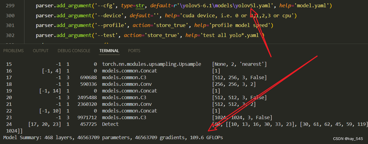
🚀运行程序,如果出现下面的内容则说明添加成功🚀
                 from  n    params  module                                  arguments
  0                -1  1      1936  models.common.VanillaStem               [3, 16, 4, 4, None, 1]
  1                -1  1      4784  models.common.VanillaBlock              [16, 64, 1, 2, None, 1]
  2                -1  1     19392  models.common.VanillaBlock              [64, 128, 1, 2, None, 1]
  3                -1  1     63360  models.common.VanillaBlock              [128, 256, 1, 2, None, 1]
  4                -1  1     33024  models.common.Conv                      [256, 128, 1, 1]
  5                -1  1         0  torch.nn.modules.upsampling.Upsample    [None, 2, 'nearest']
  6           [-1, 2]  1         0  models.common.Concat                    [1]
  7                -1  1     90880  models.common.C3                        [256, 128, 1, False]
  8                -1  1      8320  models.common.Conv                      [128, 64, 1, 1]
  9                -1  1         0  torch.nn.modules.upsampling.Upsample    [None, 2, 'nearest']
 10           [-1, 1]  1         0  models.common.Concat                    [1]
 11                -1  1     22912  models.common.C3                        [128, 64, 1, False]
 12                -1  1     36992  models.common.Conv                      [64, 64, 3, 2]
 13           [-1, 8]  1         0  models.common.Concat                    [1]
 14                -1  1     74496  models.common.C3                        [128, 128, 1, False]
 15                -1  1    147712  models.common.Conv                      [128, 128, 3, 2]
 16           [-1, 4]  1         0  models.common.Concat                    [1]
 17                -1  1    296448  models.common.C3                        [256, 256, 1, False]
 18      [11, 14, 17]  1    115005  Detect                                  [80, [[10, 13, 16, 30, 33, 23], [30, 61, 62, 45, 59, 119], [116, 90, 156, 198, 373, 326]], [64, 128, 256]]
YOLOv5_vNet summary: 137 layers, 915261 parameters, 915261 gradients, 2.2 GFLOPs
3. 完整代码分享
https://pan.baidu.com/s/1gWpg6cMyS3k7S9OXiCiw4Q?pwd=wdmw提取码: wdmw
4.GFLOPs
关于GFLOPs的计算方式可以查看:百面算法工程师 | 卷积基础知识——Convolution
未改进的GFLOPs
改进后的GFLOPs

5. 进阶
你能在不同的位置添加全局注意力机制吗?
6. 总结
VanillaNet 是一种极简主义神经网络架构,通过减少层数、简化操作以及避免复杂的连接方式(如自注意力和残差连接),实现高效的图像处理和分类。其主要原理包括:使用少量的卷积层来提取特征,采用分阶段的设计来逐步下采样特征图和增加通道数,每个阶段包含一个卷积层和一个池化层来简化计算;在训练过程中,通过深度训练策略将初始激活函数逐渐简化为恒等映射,以便合并卷积层和提高推理速度;最终,通过全连接层将高维特征映射到分类标签,从而实现简化结构下的高效分类。这种设计不仅保证了模型的性能,还优化了资源利用,使其适合在计算资源受限的环境中使用。


 990
990

 被折叠的 条评论
为什么被折叠?
被折叠的 条评论
为什么被折叠?
 到【灌水乐园】发言


