limma | 分层样本的差异分析这样搞！（二）

1写在前面

上期介绍了用limma包做配对样本的差异分析。
本期介绍一下Multi-level如何处理吧。 🥳

应用场景：Control 和 Diseased的T细胞和B细胞分层对比。

2用到的包

rm(list = ls())
library(tidyverse)
library(limma)
library(GEOquery)

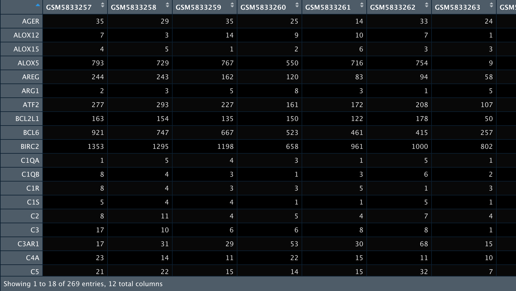
3示例数据

这里我们还是利用上期介绍的GEO数据库上的dataset。😘
在3个样本中对T细胞和B细胞分别进行了转录组分析。
每个样本的细胞都分为Control或anti-BTLA组。

GSE194314 <- getGEO('GSE194314', destdir=".",getGPL = F)
exprSet <- exprs(GSE194314[[1]]) 
exprSet <- normalizeBetweenArrays(exprSet) %>% 
  log2(.)

4获取分组数据

pdata <- pData(GSE194314[[1]])

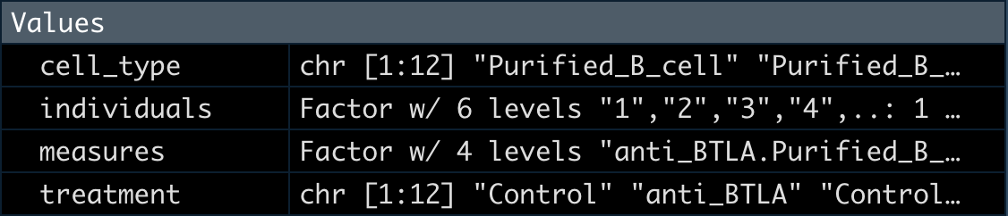
5整理分组数据

这里我们提取出分组数据后转为factor。

individuals <- factor(unlist(lapply(pdata$characteristics_ch1.1,function(x) strsplit(as.character(x),": ")[[1]][2])))

cell_type <- factor(unlist(lapply(pdata$characteristics_ch1,function(x) strsplit(as.character(x),": ")[[1]][2])))
cell_type <- gsub("[[:punct:]]","", cell_type)
cell_type <- gsub("\\s","_", cell_type)

treatment <- unlist(lapply(pdata$characteristics_ch1.2,function(x) strsplit(as.character(x),": ")[[1]][2]))

treatment <- factor(treatment,levels = unique(treatment))

treatment<- gsub("-", "_", treatment)

6Multi-level的处理与理解

6.1 整理分组矩阵

如果我们的目的是比较两种细胞类型间的差异，可以在样本内部进行，因为每个样本都会产生两种细胞类型的值。 🧐
如果我们想将Control与anti-BTLA进行比较，这种比较就是在不同样本之间进行了。

这里大家可以理解为，需要进行组内和组间比较，处理样本时需要用到random effect，在limma包中需要调用duplicateCorrelation函数进行处理。😲

measures <- factor(paste(treatment, cell_type,sep="."))

design <- model.matrix(~ 0 + measures)

colnames(design) <- levels(measures)

---

6.2 相关性计算

然后，我们在同一样本上计算不同组学间的相关性。

corfit <- duplicateCorrelation(exprSet, design, block = individuals)
corfit$consensus

---

6.3 模型拟合

fit <- lmFit(exprSet, design, block = individuals, correlation = corfit$consensus)

---

6.4 设置比较组

这里我们设置一下比较组，用-分隔。👐

cm <- makeContrasts(antiBLTA_vs_Control_For_Bcell = 
                      anti_BTLA.Purified_B_cell-Control.Purified_B_cell,
                    
                    antiBLTA_vs_Control_For_Tcell = 
                    anti_BTLA.Purified_CD4_T_cell-Control.Purified_CD4_T_cell,  
                    
                    Bcell_vs_Tcell_For_Control = 
                   Control.Purified_B_cell-Control.Purified_CD4_T_cell,  
                   
                    Bcell_vs_Tcell_For_antiBLTA = 
                    anti_BTLA.Purified_B_cell-anti_BTLA.Purified_CD4_T_cell,
                    levels = design )

---

6.5 差异分析

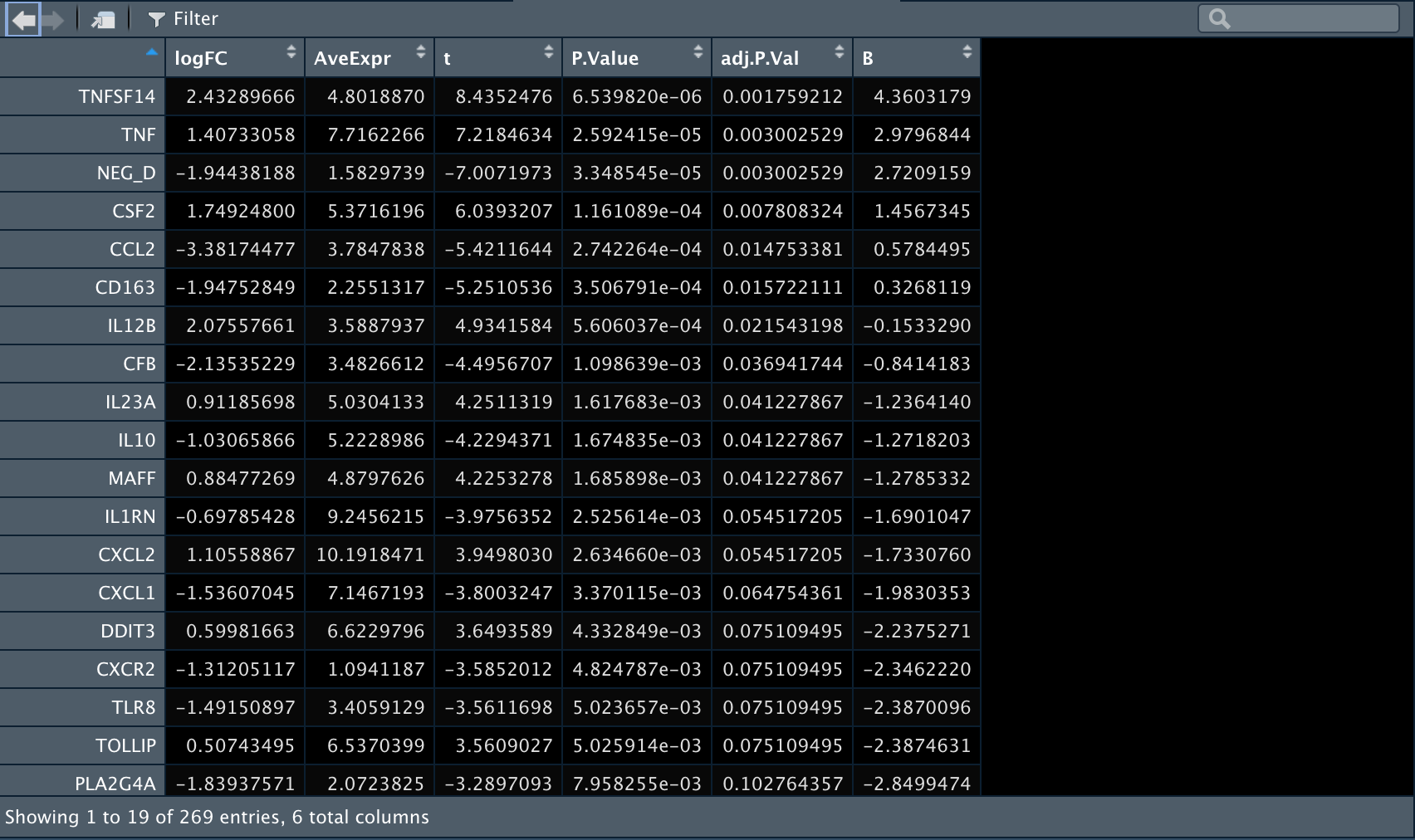
1️⃣ 现在我们比较一下在B细胞中anti-BLTA组和Control组之间的差异表达基因。

fit2 <- contrasts.fit(fit, cm)
fit2 <- eBayes(fit2)

res_antiBLTA_vs_Control_For_Bcell <- topTable(fit2, 
                coef = "antiBLTA_vs_Control_For_Bcell",
                n = Inf,
                #p.value = 0.05
                )

---

2️⃣ 再比较一下在T细胞中anti-BLTA组和Control组之间的差异表达基因。

res_antiBLTA_vs_Control_For_Tcell <- topTable(fit2, 
                coef = "antiBLTA_vs_Control_For_Tcell",
                n = Inf,
                #p.value = 0.05
                )

---

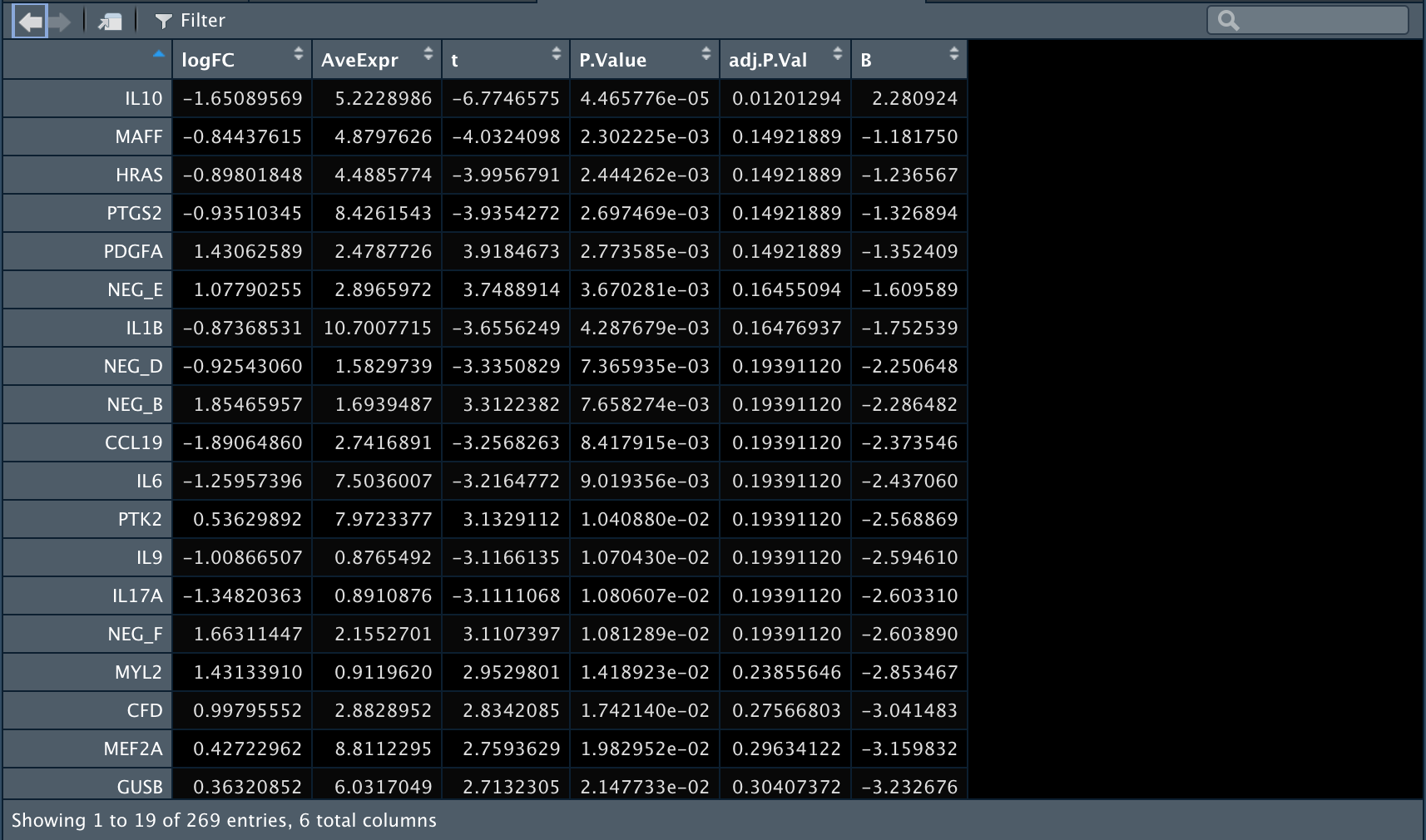
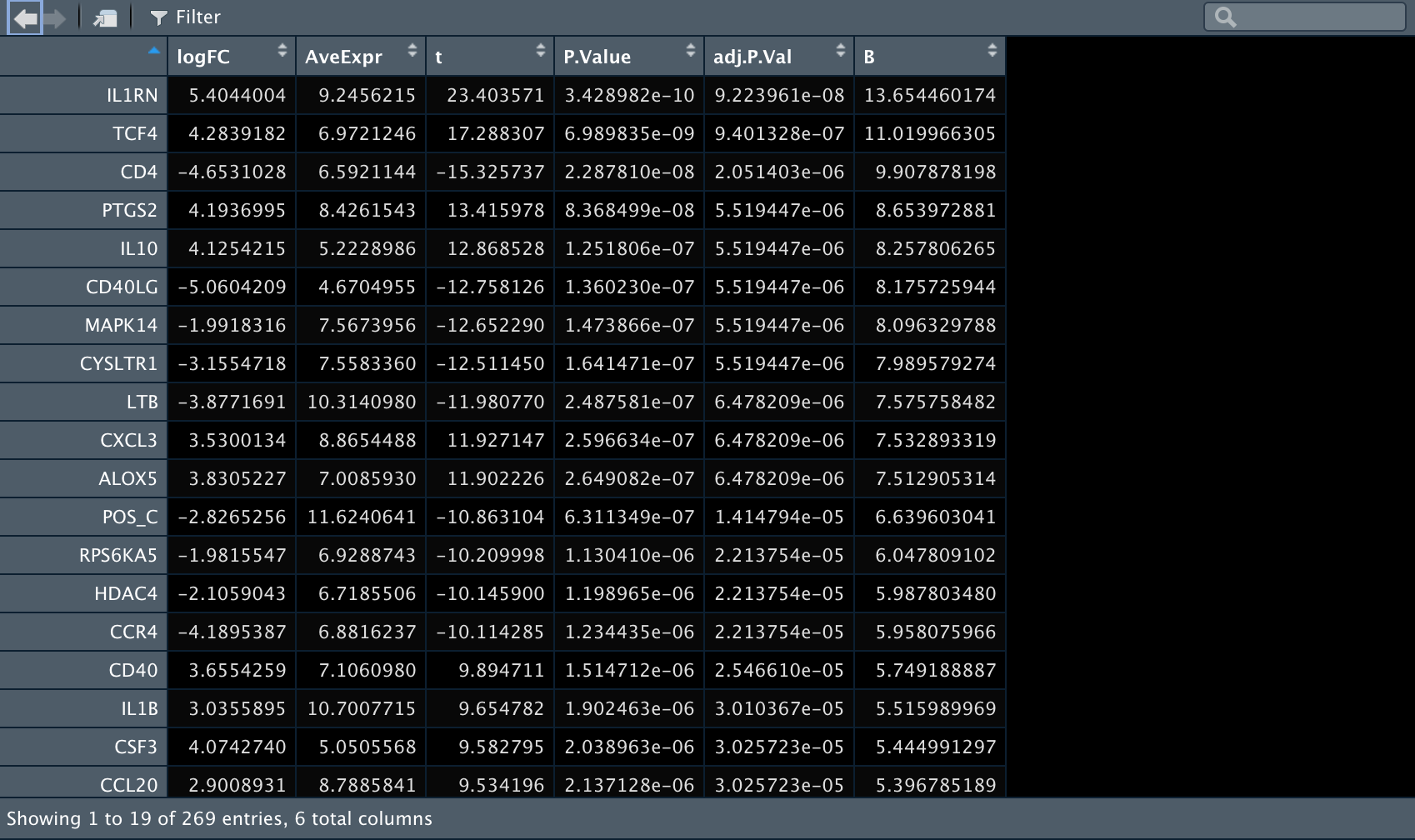
3️⃣ 再比较一下Control组内T细胞和B细胞之间的差异表达基因。

res_Bcell_vs_Tcell_For_Control <- topTable(fit2, 
                coef = "Bcell_vs_Tcell_For_Control",
                n = Inf,
                #p.value = 0.05
                )

---

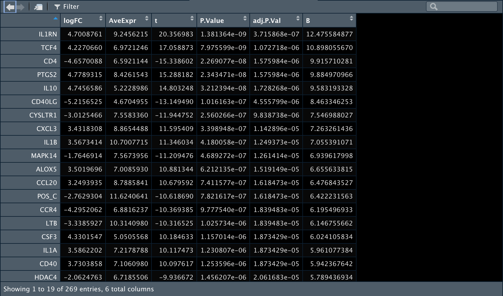
4️⃣ 再比较一下anti-BLTA组内T细胞和B细胞之间的差异表达基因。

res_Bcell_vs_Tcell_For_antiBLTA <- topTable(fit2, 
                coef = "Bcell_vs_Tcell_For_antiBLTA",
                n = Inf,
                #p.value = 0.05
                )

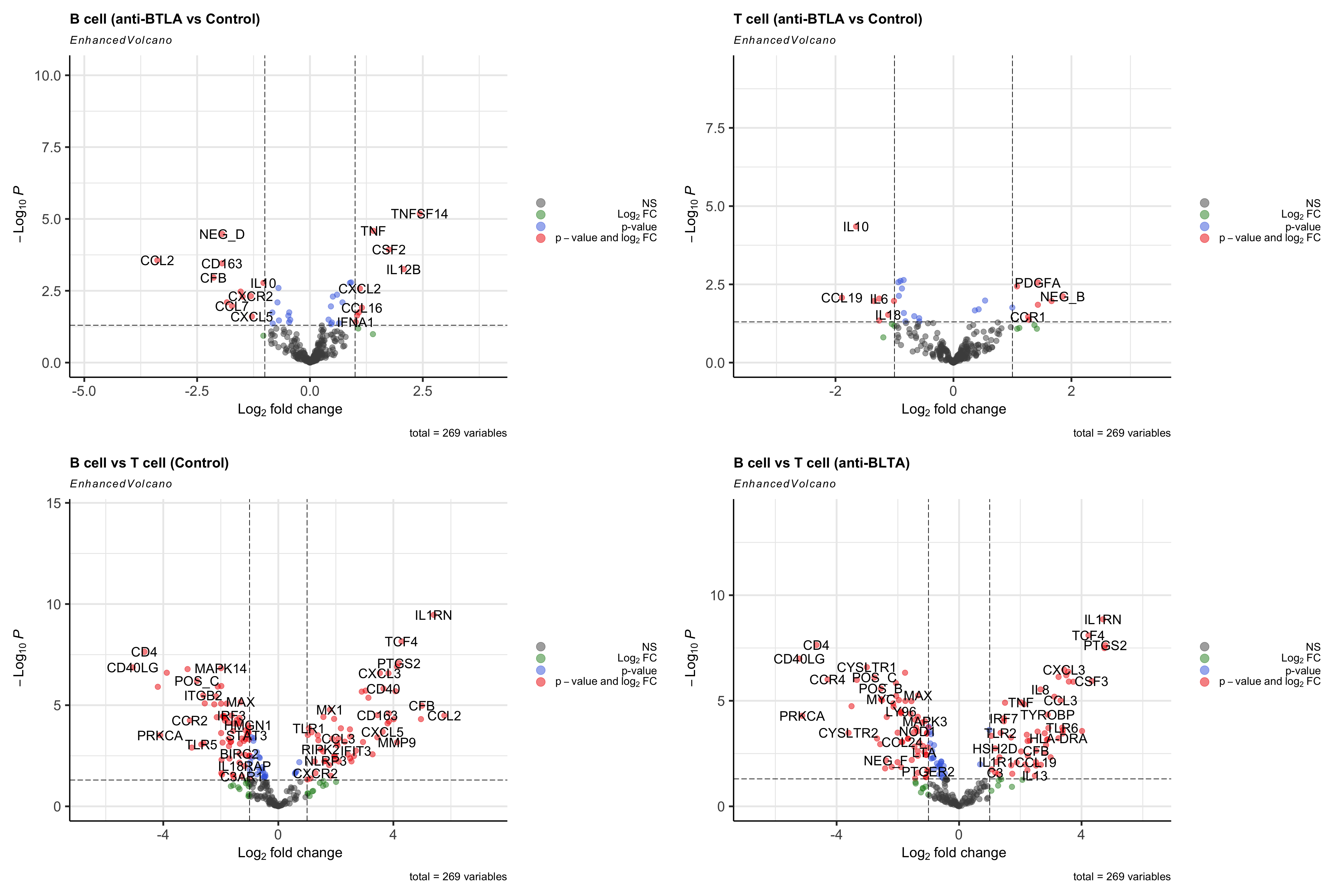
7可视化

我们直接用火山图可视化对比一下吧。🤒 这里我们把阈值设置为|logFC|>1，pvalue<0.05。

library(EnhancedVolcano)
library(patchwork)

p1 <- EnhancedVolcano(res_antiBLTA_vs_Control_For_Bcell,
    lab = rownames(res_antiBLTA_vs_Control_For_Bcell),
    x = 'logFC',
    y =  'P.Value',
    title = 'B cell (anti-BTLA vs Control)',
    pointSize = 3.0,
    labSize = 6.0,
    legendPosition = 'right',
    pCutoff = 0.05,
    FCcutoff = 1)
  

p2 <- EnhancedVolcano(res_antiBLTA_vs_Control_For_Tcell,
    lab = rownames(res_antiBLTA_vs_Control_For_Tcell),
    x = 'logFC',
    y =  'P.Value',
    title = 'T cell (anti-BTLA vs Control)',
    pointSize = 3.0,
    labSize = 6.0,
    legendPosition = 'right',
    pCutoff = 0.05,
    FCcutoff = 1)

p3 <- EnhancedVolcano(res_Bcell_vs_Tcell_For_Control,
    lab = rownames(res_Bcell_vs_Tcell_For_Control),
    x = 'logFC',
    y =  'P.Value',
    title = 'B cell vs T cell (Control)',
    pointSize = 3.0,
    labSize = 6.0,
    legendPosition = 'right',
    pCutoff = 0.05,
    FCcutoff = 1)

p4 <- EnhancedVolcano(res_Bcell_vs_Tcell_For_antiBLTA,
    lab = rownames(res_Bcell_vs_Tcell_For_antiBLTA),
    x = 'logFC',
    y =  'P.Value',
    title = 'B cell vs T cell (anti-BLTA)',
    pointSize = 3.0,
    labSize = 6.0,
    legendPosition = 'right',
    pCutoff = 0.05,
    FCcutoff = 1)


wrap_plots(p1,p2,p3,p4)

---

最后祝大家早日不卷!~

---

点个在看吧各位~ ✐.ɴɪᴄᴇ ᴅᴀʏ 〰

本文由 mdnice 多平台发布