鲸鱼优化算法（WOA）

• 一、基本原理
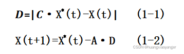
  标准 WOA 模拟了座头鲸特有的搜索方法和围捕机制，主要包括：围捕猎物、气泡网捕食、搜索猎物三个重要阶段。WOA 中每个座头鲸的位置代表一个潜在解，通过在解空间中不断更新鲸鱼的位置，最终获得全局最优解。
  • 围捕猎物

    

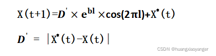
  • 气泡网捕食

    

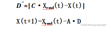
  • 搜索猎物

    

• 二、基本流程

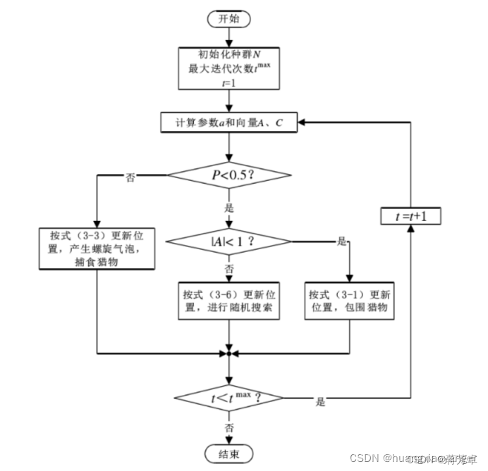
步骤 1：设置鲸鱼数量 N 和算法的最大迭代次数 tmax，初始化位置信息；
步骤 2：计算每条鲸鱼的适应度，找到当前最优鲸鱼的位置并保留；
步骤 3：计算参数 a、p 和系数向量 A、C。判断概率 p 是否小于 50%，是则直接转入步骤 4，否则采用气泡网捕食机制:按式(2-1)进行位置更新；
步骤 4：判断系数向量 A 的绝对值是否小于 1，是则包围猎物：按式（1-2）更新位置；否则全局随机搜索猎物：按式（3-1）更新位置；
​步骤 5：位置更新结束，计算每条鲸鱼的适应度，并与先前保留的最优鲸鱼的位置比较，若优于，则利用新的最优解替换;
​步骤 6：判断当前计算是否达到最大迭代次数，如果是，则获得最优解，计算结束，否则进入下一次迭代，并返回步骤 3。

• 三、python代码

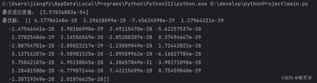
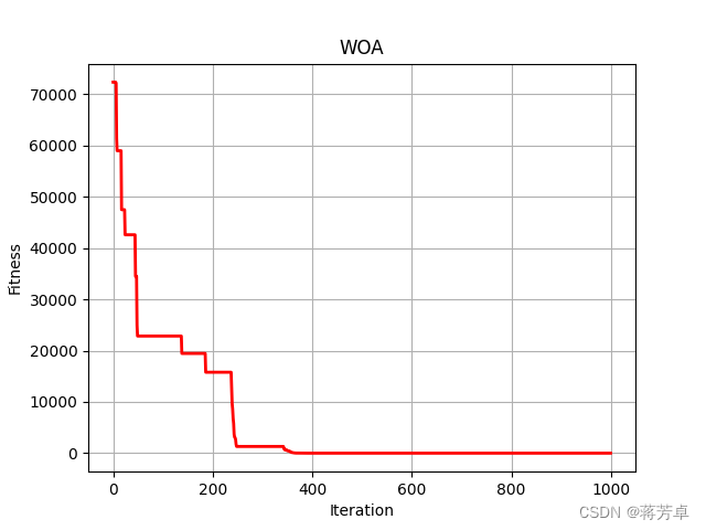
• import numpy as np
  import random
  import math
  from matplotlib import pyplot as plt
  from mpl_toolkits.mplot3d import Axes3D
  
  '''优化函数'''
  
  
  # y = x^2, 用户可以自己定义其他函数
  def fun(X):
      output = sum(np.square(X))
      return output
  
  
  ''' 种群初始化函数 '''
  
  
  def initial(pop, dim, ub, lb):
      X = np.zeros([pop, dim])
      for i in range(pop):
          for j in range(dim):
              X[i, j] = random.random() * (ub[j] - lb[j]) + lb[j]
  
      return X, lb, ub
  
  
  '''边界检查函数'''
  
  
  def BorderCheck(X, ub, lb, pop, dim):
      for i in range(pop):
          for j in range(dim):
              if X[i, j] > ub[j]:
                  X[i, j] = ub[j]
              elif X[i, j] < lb[j]:
                  X[i, j] = lb[j]
      return X
  
  
  '''计算适应度函数'''
  
  
  def CaculateFitness(X, fun):
      pop = X.shape[0]
      fitness = np.zeros([pop, 1])
      for i in range(pop):
          fitness[i] = fun(X[i, :])
      return fitness
  
  
  '''适应度排序'''
  
  
  def SortFitness(Fit):
      fitness = np.sort(Fit, axis=0)
      index = np.argsort(Fit, axis=0)
      return fitness, index
  
  
  '''根据适应度对位置进行排序'''
  
  
  def SortPosition(X, index):
      Xnew = np.zeros(X.shape)
      for i in range(X.shape[0]):
          Xnew[i, :] = X[index[i], :]
      return Xnew
  
  
  '''鲸鱼优化算法'''
  
  
  def WOA(pop, dim, lb, ub, Max_iter, fun):
      X, lb, ub = initial(pop, dim, ub, lb)  # 初始化种群
      fitness = CaculateFitness(X, fun)  # 计算适应度值
      fitness, sortIndex = SortFitness(fitness)  # 对适应度值排序
      X = SortPosition(X, sortIndex)  # 种群排序
      GbestScore = fitness[0]
      GbestPositon = np.zeros([1,dim])
      GbestPositon[0,:] = X[0, :]
      Curve = np.zeros([MaxIter, 1])
      for t in range(MaxIter):
          Leader = X[0, :]  # 领头鲸鱼
          a = 2 - t * (2 / MaxIter)  # 线性下降权重2 - 0
          a2 = -1 + t * (-1 / MaxIter)  # 线性下降权重-1 - -2
          for i in range(pop):
              r1 = random.random()
              r2 = random.random()
  
              A = 2 * a * r1 - a
              C = 2 * r2
              b = 1
              l = (a2 - 1) * random.random() + 1
  
              for j in range(dim):
  
                  p = random.random()
                  if p < 0.5:
                      if np.abs(A) >= 1:
                          rand_leader_index = min(int(np.floor(pop * random.random() + 1)), pop - 1)
                          X_rand = X[rand_leader_index, :]
                          D_X_rand = np.abs(C * X_rand[j] - X[i, j])
                          X[i, j] = X_rand[j] - A * D_X_rand
                      elif np.abs(A) < 1:
                          D_Leader = np.abs(C * Leader[j] - X[i, j])
                          X[i, j] = Leader[j] - A * D_Leader
                  elif p >= 0.5:
                      distance2Leader = np.abs(Leader[j] - X[i, j])
                      X[i, j] = distance2Leader * np.exp(b * l) * np.cos(l * 2 * math.pi) + Leader[j]
  
          X = BorderCheck(X, ub, lb, pop, dim)  # 边界检测
          fitness = CaculateFitness(X, fun)  # 计算适应度值
          fitness, sortIndex = SortFitness(fitness)  # 对适应度值排序
          X = SortPosition(X, sortIndex)  # 种群排序
          if fitness[0] <= GbestScore:  # 更新全局最优
              GbestScore = fitness[0]
              GbestPositon[0,:] = X[0, :]
          Curve[t] = GbestScore
  
      return GbestScore, GbestPositon, Curve
  
  
  '''主函数 '''
  # 设置参数
  pop = 50  # 种群数量
  MaxIter = 1000  # 最大迭代次数
  dim = 30  # 维度
  lb = -100 * np.ones([dim, 1])  # 下边界
  ub = 100 * np.ones([dim, 1])  # 上边界
  
  GbestScore, GbestPositon, Curve = WOA(pop, dim, lb, ub, MaxIter, fun)
  print('最优适应度值：', GbestScore)
  print('最优解：', GbestPositon)
  
  # 绘制适应度曲线
  plt.figure(1)
  plt.plot(Curve, 'r-', linewidth=2)
  plt.xlabel('Iteration', fontsize='medium')
  plt.ylabel("Fitness", fontsize='medium')
  plt.grid()
  plt.title('WOA', fontsize='large')
  
  # 绘制搜索空间
  fig = plt.figure(2)
  ax = Axes3D(fig)
  X = np.arange(-4, 4, 0.25)
  Y = np.arange(-4, 4, 0.25)
  X, Y = np.meshgrid(X, Y)
  Z = X ** 2 + Y ** 2
  ax.plot_surface(X, Y, Z, rstride=1, cstride=1, cmap='rainbow')
  plt.show()
  
  

  四、运行结果

•