


 本文介绍了双目视觉中利用SIFT特征点进行图像配准的方法,包括特征提取、匹配、立体匹配和图像对齐过程。强调了这种方法的鲁棒性、精度和实时性能,并提供了MATLAB代码示例,适用于机器人导航、医学图像等领域。
✅作者简介:热爱科研的Matlab仿真开发者,修心和技术同步精进,代码获取、论文复现及科研仿真合作可私信。
🍎个人主页:Matlab科研工作室
🍊个人信条:格物致知。
更多Matlab完整代码及仿真定制内容点击👇
🔥 内容介绍
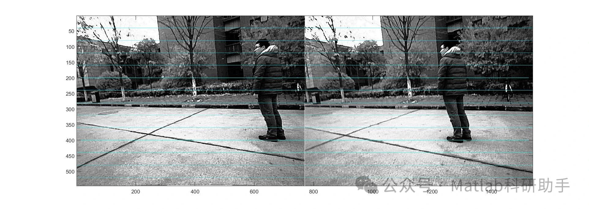
图像配准是指将两幅或多幅图像在空间上进行对齐,使它们在同一个坐标系下进行比较和分析。双目视觉是实现图像配准的一种常见方法,它利用两个摄像头采集同一场景的不同视角图像,通过特征点匹配和立体匹配算法来计算两幅图像之间的相对位姿,从而实现图像配准。
SIFT (Scale-Invariant Feature Transform) 是一种尺度不变的特征描述子,它对图像的旋转、缩放、亮度变化等具有较好的鲁棒性。在双目视觉图像配准中,SIFT特征点可以用来匹配两幅图像中的对应点,从而获得两幅图像之间的匹配关系。
基于双目视觉SIFT特征点实现图像配准的步骤如下:
-
特征提取: 对两幅图像分别提取SIFT特征点。
-
特征匹配: 利用特征描述子进行特征匹配,找到两幅图像中对应点的匹配关系。
-
立体匹配: 根据匹配关系和双目相机的参数,计算两幅图像之间的相对位姿。
-
图像配准: 根据计算出的相对位姿,将其中一幅图像进行空间变换,使其与另一幅图像对齐。
基于双目视觉SIFT特征点实现图像配准具有以下优点:
-
鲁棒性强: SIFT特征点对图像的旋转、缩放、亮度变化等具有较好的鲁棒性。
-
精度高: 双目视觉可以提供精确的深度信息,提高图像配准的精度。
-
实时性好: SIFT特征点提取和匹配算法可以快速完成,满足实时应用的需求。
总而言之,基于双目视觉SIFT特征点实现图像配准是一种高效、鲁棒的图像配准方法,它在许多领域都得到了广泛的应用,例如机器人导航、三维重建、医学图像配准等。
📣 部分代码
%%Pre Process Datads=datastore("LakeDATA\*Quality*.csv","TextType","string","DatetimeType","text");Week1=read(ds);Week1.Date= datetime(Week1.Date,'InputFormat','yyyy-MM-dd');Week1.Date.Format='dd/MM/uuuu';Week1 = rmmissing(Week1,"DataVariables",width(Week1));%% Set up the Import Options and import the dataopts = spreadsheetImportOptions("NumVariables", 3);% Specify sheet and rangeopts.Sheet = "Sheet1";opts.DataRange = "A2:C6";% Specify column names and typesopts.VariableNames = ["Parameters", "StandardValue", "IdealValue"];opts.VariableTypes = ["string", "double", "double"];% Specify variable propertiesopts = setvaropts(opts, "Parameters", "WhitespaceRule", "preserve");opts = setvaropts(opts, "Parameters", "EmptyFieldRule", "auto");% Import the dataQualityIndex = readtable("C:\Users\celeste\Desktop\fer\Proyecto Fase I\Matlab\QualityIndex.xlsx", opts, "UseExcel", false)%% Clear temporary variablesclear opts%% Analyze DataWeekdata=Week1{:,3:7};meanWeek= mean(Weekdata,'omitnan');medianWeek= median(Weekdata,'omitnan');modeWeek=mode(Weekdata);varianceWeek=var(Weekdata,'omitnan');stdWeek = std(Weekdata, 'omitnan');maxWeek= max(Weekdata);minWeek= min(Weekdata);rangeWeek= range(Weekdata);departureWeek= Weekdata-meanWeek;normalizedWeek = (Weekdata - meanWeek) ./ stdWeek;analysisTable = table(meanWeek', medianWeek', modeWeek', varianceWeek', stdWeek', maxWeek', minWeek', rangeWeek');analysisTable.Properties.VariableNames = {'Mean', 'Median', 'Mode', 'Variance', 'Standard Deviation', 'Max', 'Min', 'Range'};analysisTable.Properties.RowNames = {'Temperature', 'pH', 'TDS', 'Turbulence', 'ORP'}WeekdataTable = array2table(Weekdata, 'VariableNames', {'Temperature', 'pH', 'TDS', 'Turbidity', 'ORP'});k=sum(1./QualityIndex.StandardValue);k=1/k;Wi=(k ./QualityIndex.StandardValue);Qs=(QualityIndex.StandardValue-QualityIndex.IdealValue);for i = 1:size(WeekdataTable, 2)parameter = QualityIndex.Parameters{i};standard_value = QualityIndex.StandardValue(i);ideal_value = QualityIndex.IdealValue(i);idx = strcmp(QualityIndex.Parameters, parameter);StandardTable(:, i) = abs(standard_value-WeekdataTable(:, i));IdealTable(:,i)=abs(WeekdataTable(:,i)-ideal_value);endQt = IdealTable{:,:};StandardMatrix = table2array(StandardTable);Qi = 100*(Qt ./ StandardMatrix);QiWi=Qi.*Wi';WQI=sum(QiWi,2);Week1 = addvars(Week1, WQI, 'After', 'ORP', 'NewVariableNames', 'WQI')yfit = Ensemblemdl.predictFcn(Week1)function [trainedModel, validationRMSE] = trainRegressionModel(trainingData)% [trainedModel, validationRMSE] = trainRegressionModel(trainingData)% Returns a trained regression model and its RMSE. This code recreates the% model trained in Regression Learner app. Use the generated code to% automate training the same model with new data, or to learn how to% programmatically train models.%% Input:% trainingData: A table containing the same predictor and response% columns as those imported into the app.%%% Output:% trainedModel: A struct containing the trained regression model. The% struct contains various fields with information about the trained% model.%% trainedModel.predictFcn: A function to make predictions on new data.%% validationRMSE: A double representing the validation RMSE. In the% app, the Models pane displays the validation RMSE for each model.%% Use the code to train the model with new data. To retrain your model,% call the function from the command line with your original data or new% data as the input argument trainingData.%% For example, to retrain a regression model trained with the original data% set T, enter:% [trainedModel, validationRMSE] = trainRegressionModel(T)%% To make predictions with the returned 'trainedModel' on new data T2, use% yfit = trainedModel.predictFcn(T2)%% T2 must be a table containing at least the same predictor columns as used% during training. For details, enter:% trainedModel.HowToPredict% Auto-generated by MATLAB on 13-Apr-2024 02:26:21% Extract predictors and response% This code processes the data into the right shape for training the% model.inputTable = trainingData;predictorNames = {'Temperature', 'pH', 'TDS', 'ORP', 'WQI'};predictors = inputTable(:, predictorNames);response = inputTable.Turbulency;isCategoricalPredictor = [false, false, false, false, false];% Train a regression model% This code specifies all the model options and trains the model.template = templateTree(...'MinLeafSize', 8, ...'NumVariablesToSample', 'all');regressionEnsemble = fitrensemble(...predictors, ...response, ...'Method', 'Bag', ...'NumLearningCycles', 30, ...'Learners', template);% Create the result struct with predict functionpredictorExtractionFcn = @(t) t(:, predictorNames);ensemblePredictFcn = @(x) predict(regressionEnsemble, x);trainedModel.predictFcn = @(x) ensemblePredictFcn(predictorExtractionFcn(x));% Add additional fields to the result structtrainedModel.RequiredVariables = {'Temperature', 'pH', 'TDS', 'ORP', 'WQI'};trainedModel.RegressionEnsemble = regressionEnsemble;trainedModel.About = 'This struct is a trained model exported from Regression Learner R2023b.';trainedModel.HowToPredict = sprintf('To make predictions on a new table, T, use: \n yfit = c.predictFcn(T) \nreplacing ''c'' with the name of the variable that is this struct, e.g. ''trainedModel''. \n \nThe table, T, must contain the variables returned by: \n c.RequiredVariables \nVariable formats (e.g. matrix/vector, datatype) must match the original training data. \nAdditional variables are ignored. \n \nFor more information, see <a href="matlab:helpview(fullfile(docroot, ''stats'', ''stats.map''), ''appregression_exportmodeltoworkspace'')">How to predict using an exported model</a>.');% Extract predictors and response% This code processes the data into the right shape for training the% model.inputTable = trainingData;predictorNames = {'Temperature', 'pH', 'TDS', 'ORP', 'WQI'};predictors = inputTable(:, predictorNames);response = inputTable.Turbulency;isCategoricalPredictor = [false, false, false, false, false];% Perform cross-validationpartitionedModel = crossval(trainedModel.RegressionEnsemble, 'KFold', 5);% Compute validation predictionsvalidationPredictions = kfoldPredict(partitionedModel);% Compute validation RMSEvalidationRMSE = sqrt(kfoldLoss(partitionedModel, 'LossFun', 'mse'));end
⛳️ 运行结果
🔗 参考文献
[1]李瑞.基于图像拼接技术的双目视觉研究[D].华中科技大学[2024-04-27].DOI:10.7666/d.d085931.
🎈 部分理论引用网络文献,若有侵权联系博主删除
🎁 关注我领取海量matlab电子书和数学建模资料
👇 私信完整代码和数据获取及论文数模仿真定制
1 各类智能优化算法改进及应用
生产调度、经济调度、装配线调度、充电优化、车间调度、发车优化、水库调度、三维装箱、物流选址、货位优化、公交排班优化、充电桩布局优化、车间布局优化、集装箱船配载优化、水泵组合优化、解医疗资源分配优化、设施布局优化、可视域基站和无人机选址优化、背包问题、 风电场布局、时隙分配优化、 最佳分布式发电单元分配、多阶段管道维修、 工厂-中心-需求点三级选址问题、 应急生活物质配送中心选址、 基站选址、 道路灯柱布置、 枢纽节点部署、 输电线路台风监测装置、 集装箱船配载优化、 机组优化、 投资优化组合、云服务器组合优化、 天线线性阵列分布优化、CVRP问题、VRPPD问题、多中心VRP问题、多层网络的VRP问题、多中心多车型的VRP问题、 动态VRP问题、双层车辆路径规划(2E-VRP)、充电车辆路径规划(EVRP)、油电混合车辆路径规划、混合流水车间问题、 订单拆分调度问题、 公交车的调度排班优化问题、航班摆渡车辆调度问题、选址路径规划问题
2 机器学习和深度学习方面
2.1 bp时序、回归预测和分类
2.2 ENS声神经网络时序、回归预测和分类
2.3 SVM/CNN-SVM/LSSVM/RVM支持向量机系列时序、回归预测和分类
2.4 CNN/TCN卷积神经网络系列时序、回归预测和分类
2.5 ELM/KELM/RELM/DELM极限学习机系列时序、回归预测和分类
2.6 GRU/Bi-GRU/CNN-GRU/CNN-BiGRU门控神经网络时序、回归预测和分类
2.7 ELMAN递归神经网络时序、回归\预测和分类
2.8 LSTM/BiLSTM/CNN-LSTM/CNN-BiLSTM/长短记忆神经网络系列时序、回归预测和分类
2.9 RBF径向基神经网络时序、回归预测和分类


 3万+
3万+

 被折叠的 条评论
为什么被折叠?
被折叠的 条评论
为什么被折叠?
 到【灌水乐园】发言


