《graph self- supervised learning：a survey》论文阅读

2022.5.5 天气晴。

一、介绍

图上的深度学习多数关注于半监督学习/监督学习，但是对标签具有很严重的依赖性、泛化能力弱、鲁棒性弱，所以SSL(自监督学习)成为了一个promising的研究方向。

标签依赖性：标签的人工成本大，数据集大、领域知识多。
泛化能力弱：由于标签的存在很容易导致过拟合。
鲁棒性弱：对label-related的对抗攻击很脆弱。

在SSL中，模型通过一系列的手工辅助任务来进行学习（pretext tasks），这样监督信号就可以通过模型本身来获得，而不依赖于手工的标签，SSL这样使得模型可以获得informative representation。

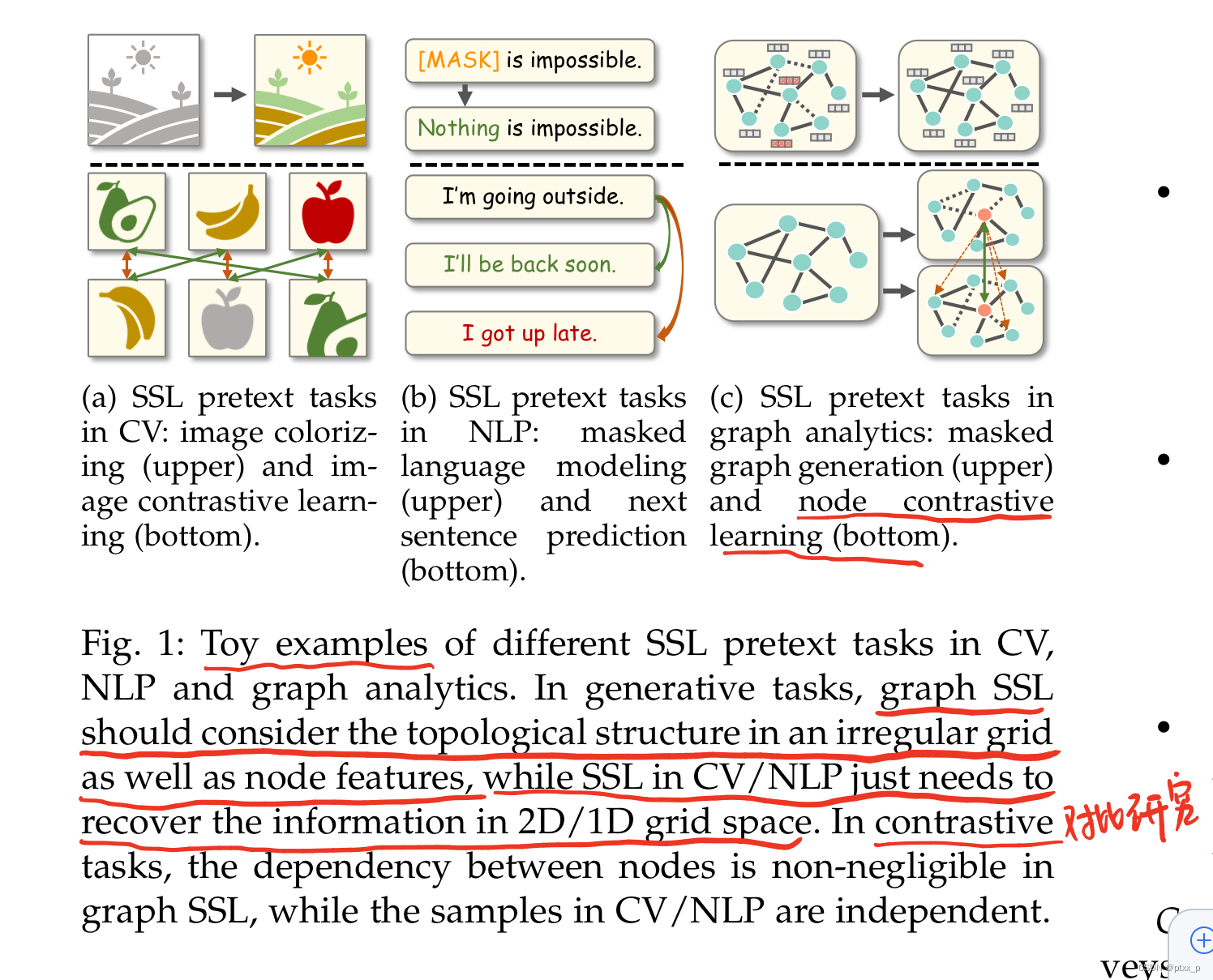
SSL on CV、NLP与SSL on graph的gap（Fig. 1）：
graph是不规则的非欧几里得结构。因此一些pretext的设计for网格结构数据不能够直接映射到图数据上来。更进一步的，图中的节点与拓扑结构紧密关联，但是在image和text中两者是分开的。因此如何处理这种关联也成为了设计pretext任务的challenge。

二、重要定义

手工标签vs伪标签：
手工标签：手工标注。
伪标签：算法自动根据数据生成，多在SSL中用来增强表示学习。

downstream tasks vs pretext tasks：
downstream tasks一般用来评测获得的graph embedding效果如何，如图分类和节点分类等。而pretext tasks则是用来帮助学习获得更好的representations，benifits downstream tasks。一般的，downstream tasks需要手工标签、pretext tasks需要伪标签。

自监督学习：
是无监督学习的一个subset，自监督学习指监督信息从data本身获取，模型通过pretext任务来获得更好的表现和泛化性能用于downstream tasks。

plain graph:
无属性、静态、同质图。G=(V,E)。

attributed graph：
节点或者是边具有属性。G=(V,E,X)。

很多GNN都使用了一个encoder的backbone，把节点特征变为节点表示（利用节点的联通关系等），readout函数常常用于根据节点表示来获得图级别的表示。

三、框架与分类

3.1 框架定义

encoder-decoder框架for graph SSL：
encoder $f_{\theta }$用于学习low- dimensional representation(aka embedding):$h_i\in H$。

pretext decoder $p_{\varphi }$：接收$H$为输入for pretext tasks。$p_{\theta }$的结构依据具体的下游任务。

graph SSL可以被定义如下：
$${\theta }^{\ast },{\varphi }^{\ast }={\mathrm{argmin}}_{\theta ,\varphi }{\mathcal{L}}_{ssl}(f_{\theta },p_{\varphi },\mathcal{D}).\text{\hspace{1em}(1)}$$
$\mathcal{D}$代表图数据分布，${\mathcal{L}}_{ssl}$代表SSL 损失函数。

通过使用学习到的graph encoder $f_{{\theta }^{\ast }}$，生成的representation可以被用于各种的下游任务。定义一个下游任务decoder $q_{\psi }$，将下游任务视为一个图supervised learning task:$${\theta }^{\ast \ast },{\psi }^{\ast }={\mathrm{argmin}}_{{\theta }^{\ast },\psi }{\mathcal{L}}_{sup}(f_{{\theta }^{\ast }},q_{\psi },\mathcal{G},y).\text{\hspace{1em}(2)}$$
$y$:下游任务的标签，${\mathcal{L}}_{sup}$有监督损失函数用于下游任务。

3.2 图自监督学习的四种分类

通过使用不同的pretext decoders和objective functions，有四种分类：generation-based，auxiliary property-based，contrastive-based，hybrid methods.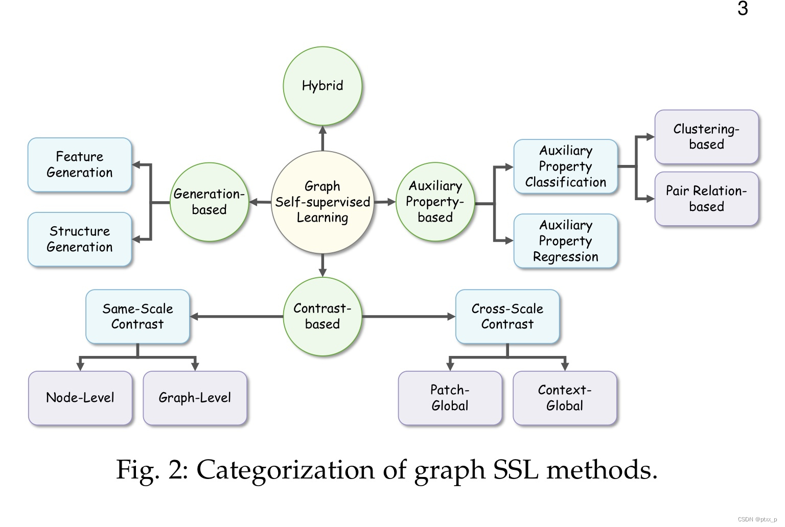


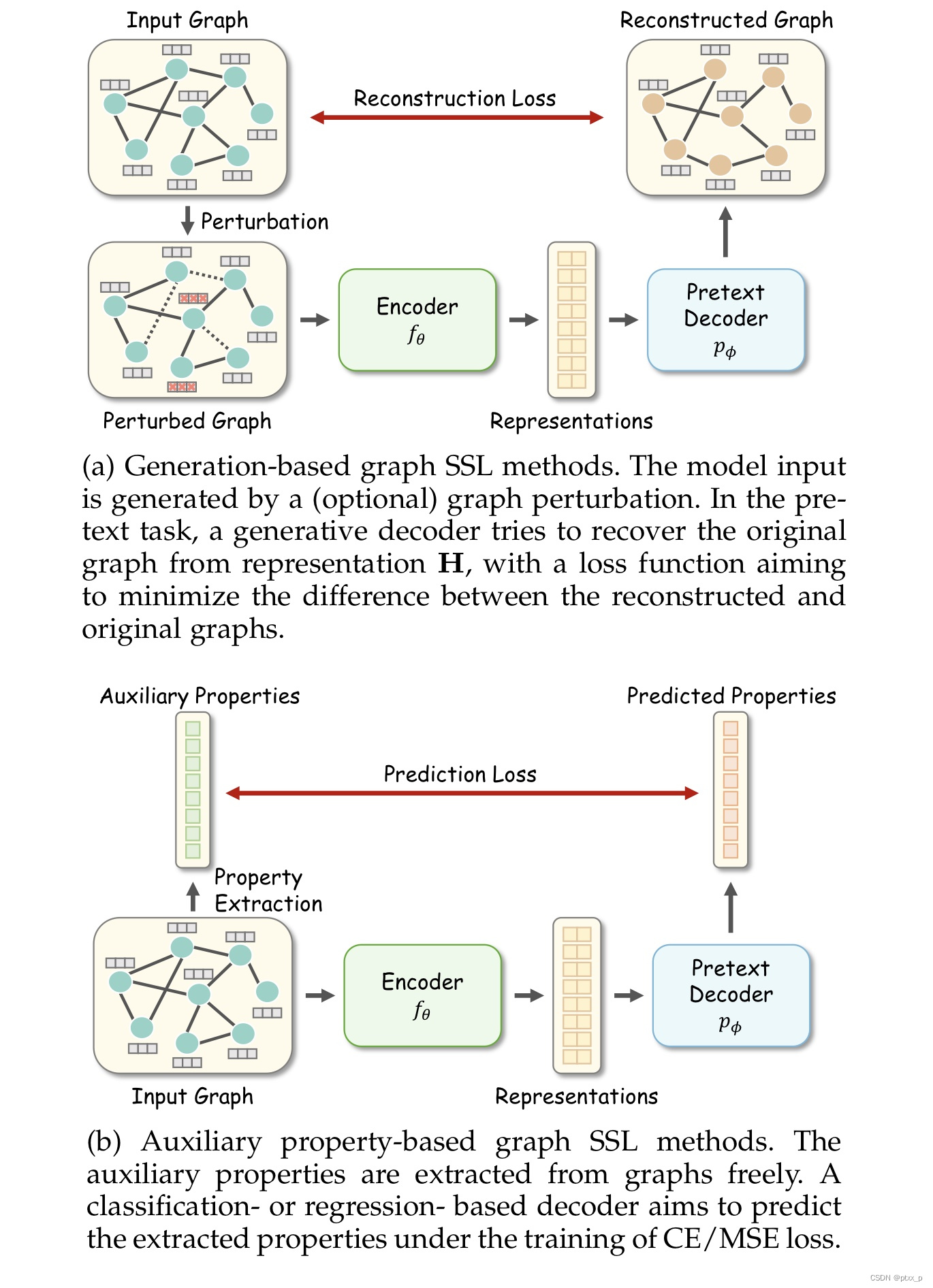
generation-based methods：
pretext task：图数据重构（图数据包括：node/edge特征和图的拓扑结构）。
可以重写公式（1）如下：
$${\theta }^{\ast },{\varphi }^{\ast }={\mathrm{argmin}}_{\theta ,\varphi }{\mathcal{L}}_{ssl}(p_{\varphi }(f_{\theta }(\tilde{\mathcal{G}})),\mathcal{G}).$$

此时${\mathcal{L}}_{ssl}$一般用于测量重构图数据和原图数据的差距。

auxiliary property-based methods：
这种方法可以被进一步分类为：regression- and classification-based。
$${\theta }^{\ast },{\varphi }^{\ast }={\mathrm{argmin}}_{\theta ,\varphi }{\mathcal{L}}_{ssl}(p_{\varphi }(f_{\theta }(\mathcal{G})),c).$$
$c$代表specific crafted auxiliary properties。对于regression-based方法，$c$可以是localized or global graph properties，如节点度或者到cluster的距离，此时${\mathcal{L}}_{ssl}$可以是MSE。对于classification-based方法，auxiliary properties可以是伪标签，如图切分或者cluster的下标，此时${\mathcal{L}}_{ssl}$可以是CE。

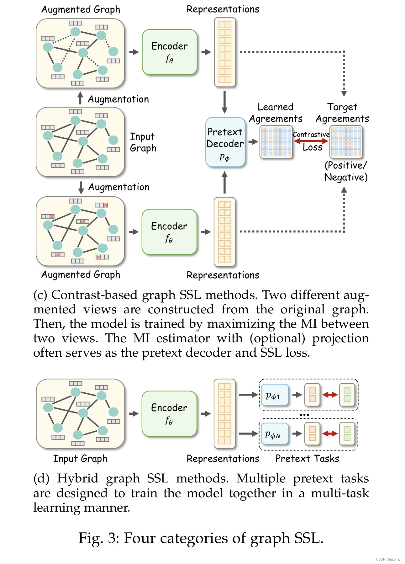
contrast-based methods：
基于互信息最大化的思想出发（mutual information maximization）。
$${\theta }^{\ast },{\varphi }^{\ast }={\mathrm{argmin}}_{\theta ,\varphi }{\mathcal{L}}_{ssl}(p_{\varphi }(f_{\theta }({\tilde{\mathcal{G}}}^{(1)},{\tilde{\mathcal{G}}}^{(2)})))).$$
其中${\tilde{\mathcal{G}}}^{(1)},{\tilde{\mathcal{G}}}^{(2)}$ 是不同的对图的增强视角。
pretext decoder $p_{\varphi }$是一个discriminator（如bilinear function or dot product），${\mathcal{L}}_{ssl}$是对比损失。
pretext task目标是：估计和最大化MI between positive pairs/最小化MI between negative pairs。

hybrid methods：
可能组合了之前提到的多种方法，可能是weighted or unweighted combination。

讨论：
generation-based methods：simple to implement，but memory-consuming for large scale graph。
auxiliary property-based methods：the selection of 有用的附加属性需要领域知识。
contrast-based methods：more flexible designs and boarder applications。对比学习框架、增强策略和损失函数设计需要大量时间的实验。
hybrid methods：main challenge is：如何设计一个协同训练框架来balance每个成分。

3.3 自监督训练策略的分类

根据graph encoders，self-supervised pretext tasks，downstream tasks之间的关系，图自监督训练方法大致可以分为：
pre-training and fine-tuning（PF）、joint learning(JL)、 unsupervised representation learning(URL).

pre-training and fine-tuning（PF）：

1. encoder $f_{\theta }$首先在pre- training数据集上通过pretext tasks进行pre-train，这可以被视为是对encoder参数的初始化。
2. the pre-trained encoder $f_{{\theta }_{init}}$在fine-tuning数据集上with a downstream decoder $q_{\psi }$ under supervision of specific downstraem tasks进行fine-tune。

$${\theta }^{\ast },{\varphi }^{\ast }={\mathrm{argmin}}_{\theta ,\varphi }{\mathcal{L}}_{ssl}(f_{\theta },p_{\varphi },\mathcal{D})$$.
$${\theta }^{\ast \ast },{\varphi }^{\ast }={\mathrm{argmin}}_{{\theta }^{\ast },\psi }{\mathcal{L}}_{sup}(f_{\theta },q_{\psi },\mathcal{G},y)$$

pre-training和fine-tuning的数据集可以是一致的或者不一致的。

joint learning(JL):
$\alpha$为一个trade-off超参数，JL可以被视为是一种multi-task learning，pretext task可以被视为是一种对downstraem task的regularization：
$${\theta }^{\ast },{\varphi }^{\ast },{\psi }^{\ast }={\mathrm{argmin}}_{\theta ,\varphi ,\psi }[\alpha {\mathcal{L}}_{ssl}(f_{\theta },p_{\varphi },\mathcal{D})+{\mathcal{L}}_{sup}(f_{\theta },q_{\psi },\mathcal{G},y)].$$

unsupervised representation learning(URL):
URL 策略的第一步几乎和PF是一样的。两者的不同在于：

1. 第二步的encoder的参数frozen了（在下游任务的训练过程中）。
2. 这两步的训练使用相同的数据集。

$${\theta }^{\ast },{\varphi }^{\ast }={\mathrm{argmin}}_{\theta ,\varphi }{\mathcal{L}}_{ssl}(f_{\theta },p_{\varphi },\mathcal{D})$$.
$${\varphi }^{\ast }={\mathrm{argmin}}_{\psi }{\mathcal{L}}_{sup}(f_{\theta }^{\ast },q_{\psi },\mathcal{G},y)$$
和其他策略相比，URL更加具有挑战性，因为在encoder的训练过程中无监督信息（因为encoder参数被冻结了）。

3.4 下游任务的分类

下游任务可以被大致分为：node-、link-、graph-level tasks。

四、generation-based methods

可以大致被分为：feature generation、structure generation。

4.1 feature generation

feature generation：learn by recovering feature information from the perturbed or original graphs。
$${\theta }^{\ast },{\varphi }^{\ast }={\mathrm{argmin}}_{\theta ,\varphi }{\mathcal{L}}_{mse}(p_{\varphi }(f_{\theta }(\tilde{\mathcal{G}})),\hat{X}).$$
其中，$p_{\varphi }(\cdot )$is the decoder for feature regression（如：一个全连接网络用于maps： representations -> reconstructed features）
$\hat{X}$是各种feature matrices的通用表示。

为了利用节点之间的依赖性，一种具有代表性的特征生成的branch follows the masked feature regression strategy.
举例：graph completion：$\hat{X}=X,\tilde{\mathcal{G}}=(A,\tilde{X})$.
attibutedMask：$\hat{X}=PCA(X)$,因此还原高维稀疏的raw data是很困难的.
attrMasking：$\hat{X}=[X,X_{edge}]$.

另一种代表性的branch是利用noisy features。$\tilde{\mathcal{G}}=(A,\tilde{X})$，其中$\tilde{X}$ is corrupted with random noise。

还可以直接使用clean data 来 rebuilding features.$\tilde{\mathcal{G}}=(A,X).$

4.2 structure generation

learn by recovering the structural information。在多数情况下，都是重构邻接矩阵。
$${\theta }^{\ast },{\varphi }^{\ast }={\mathrm{argmin}}_{\theta ,\varphi }{\mathcal{L}}_{ssl}(p_{\varphi }(f_{\theta }(\tilde{\mathcal{G}})),A).$$
$p_{\varphi }(\cdot )$ is a decoder for结构重建，$A$为部分或者全部的邻接矩阵。

邻接矩阵中存在的边一般为positive sample，不存在的为negative。为了避免稀疏邻接矩阵的unbalanced问题：1.re-weighting $A_{i,j}=1$的系数。 2.sub- sampling terms with $A_{i,j}=0$.

两大类：rebuilding the full graph / reconstruct the masked edges。

讨论：
structure generation：更多利用node pair-level information。
feature generation：更多利用node level knowledge。

五、auxiliary property-based methods

auxiliary property-based methods从node-、link-、graph- level properties来获得监督信息。和监督学习是几乎一样的训练模式：learn with sample-label pairs。但是监督学习里的标签是手工标签，而auxiliary property-based methods是伪标签：self-generated automatically without any cost。大致可以分为两类：auxiliary property classification、auxiliary property regression。

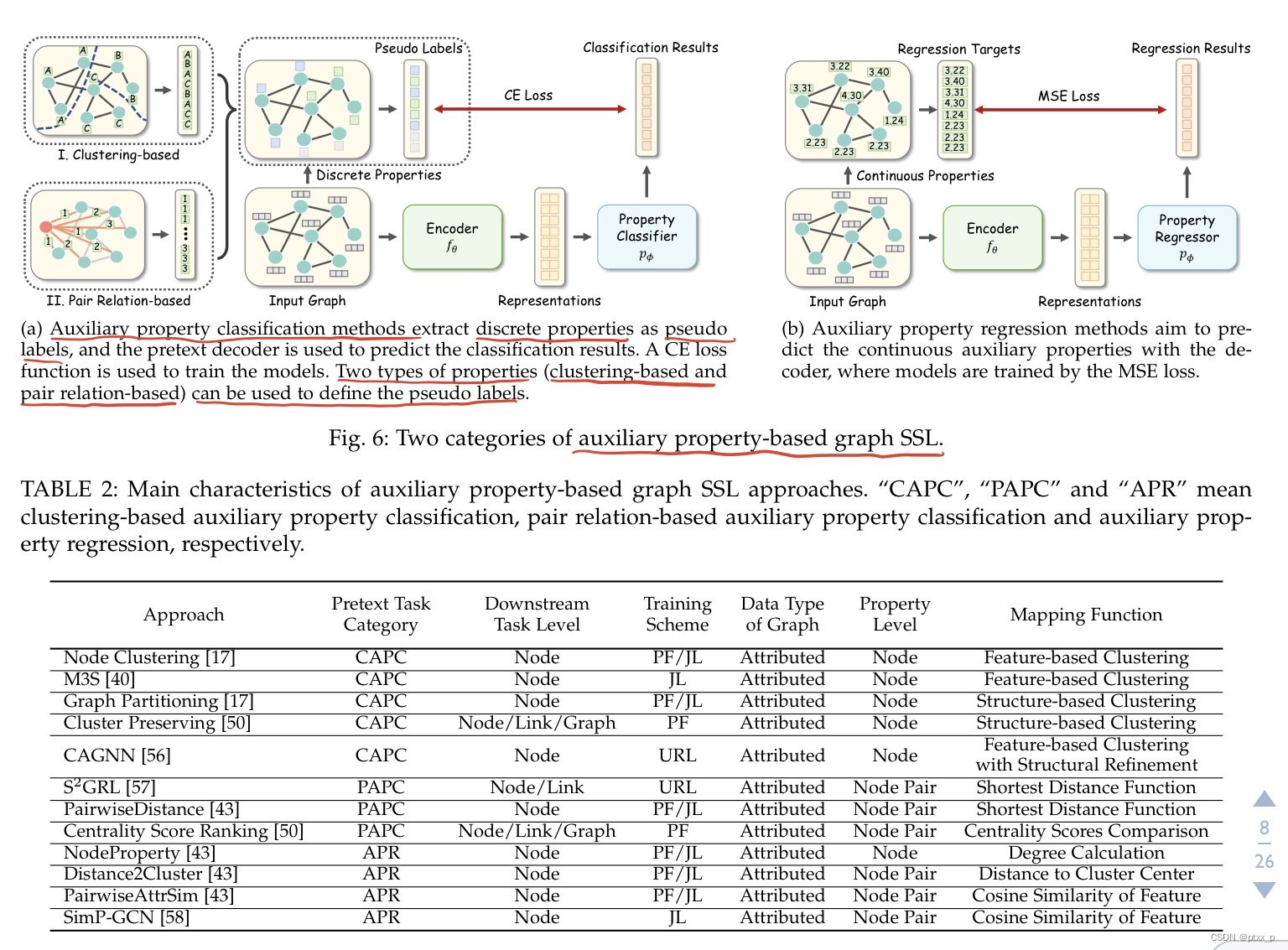
5.1 auxiliary property classification

$${\theta }^{\ast },{\varphi }^{\ast }={\mathrm{argmin}}_{\theta ,\varphi }{\mathcal{L}}_{ssl}(p_{\varphi }(f_{\theta }(\mathcal{G})),c).$$
其中$p_{\varphi }$ 是基于神经网络分类器的decoder，输出是一个k维的概率向量（k为类别的数目），$c$是相关的伪标签（属于伪标签集合$C$）。根据伪标签集合$C$的不同，大致可以分为两类：clustering-based、pair relation-based method。

5.1.1 clustering-based methods

a promising way to construct 伪标签：根据节点特征和结构属性将节点划分为不同的clusters。
mapping function ：$\Omega :V\to C$,用于为每个节点获得伪标签，一般基于无标签聚类或者是切分算法。
learning objective：
$${\theta }^{\ast },{\varphi }^{\ast }={\mathrm{argmin}}_{\theta ,\varphi }\frac{1}{|V|}\sum _{v_i\in V}{\mathcal{L}}_{ce}(p_{\varphi }([f_{\theta }(\mathcal{G}){]}_{v_i}),\Omega (v_i)).$$
其中，$[\cdot {]}_{v_i}$代表the picking function to extract the representation of $v_i.$

feature-based clustering：by feature-based clustering algorithm。
structure-based clustering：by minimizing the connections across subsets。

5.1.2 pair relation-based methods

关注于：the relationship between each pair of nodes within a graph。输入是：a pair of nodes。
mapping function ：$\Omega :V\times V\to C$,用于根据pair-wise contextual relationship来获得伪标签。
objective function：
$${\theta }^{\ast },{\varphi }^{\ast }={\mathrm{argmin}}_{\theta ,\varphi }\frac{1}{|P|}\sum _{v_i,v_j\in P}{\mathcal{L}}_{ce}(p_{\varphi }([f_{\theta }(\mathcal{G}){]}_{v_i,v_j}),\Omega (v_i,v_j)).$$
$P\subseteq V\times V$：node pair set defined by specific tasks.
$[\cdot {]}_{v_i,v_j}$：picking function that extracts and concats the node representations of $v_i,v_j.$

5.2 auxiliary property regression

和auxiliary property classification相比，auxiliary properties是一定范围内的连续值（而不是一个有限集合里的离散伪标签）。
$${\theta }^{\ast },{\varphi }^{\ast }={\mathrm{argmin}}_{\theta ,\varphi }{\mathcal{L}}_{mse}(p_{\varphi }(f_{\theta }(\mathcal{G})),c).$$
$c\in \mathbb{R}$ 是一个连续的属性值。这种属性值可以是节点度、local node importance，local clustering coefficient。
以节点度举例：
$${\theta }^{\ast },{\varphi }^{\ast }={\mathrm{argmin}}_{\theta ,\varphi }\frac{1}{|V|}\sum _{v_i\in V}{\mathcal{L}}_{mse}(p_{\varphi }([f_{\theta }(\mathcal{G}){]}_{v_i}),\Omega (v_i)).$$
$\Omega (v_i)={\sum }_{j=1}^n{A}_{ij}.$
也可以利用pair-wise property作为回归目标：
$${\theta }^{\ast },{\varphi }^{\ast }={\mathrm{argmin}}_{\theta ,\varphi }\frac{1}{|P|}\sum _{v_i,v_j\in P}{\mathcal{L}}_{mse}(p_{\varphi }([f_{\theta }(\mathcal{G}){]}_{v_i,v_j}),\Omega (v_i,v_j)).$$
举例：$\Omega (v_i,v_j)=cosine(v_i,v_j)$:the cosine similarity of raw features。

讨论：classification的方法比regression更多，因为有很多的定义离散伪标签的方法。更多连续属性的应用研究can be future direction。

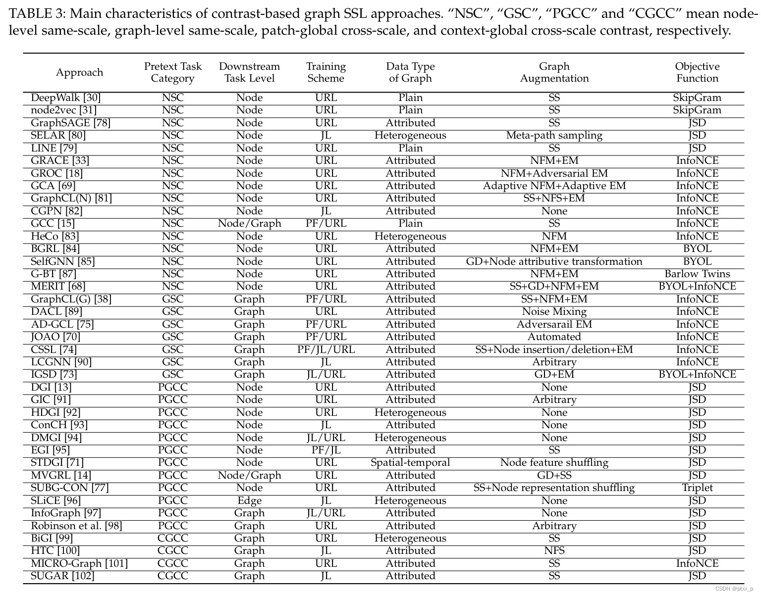
六、contrast-based methods

基于对比的方法基于the idea of 互信息最大化（mutual information maximization），learns by predicting the agreement between two augmented instances。

存在各种各样的图增强和对比学习的pretext tasks。可以分为三个部分来讲解说明这种方法。
1.graph augmentation：用于生成各种各样的graph instances。
2.graph contrastive learning：在非欧几里得空间中生成各种各样的contrastive pretext tasks。
3.mutual information estimation：measures the MI between instances and forms the contrastive learning objective together with specific pretext tasks。

6.1 graph augmentations

现在的图增强方法大致可以被分为：attributive-based、topological-based、hybrid augmentations。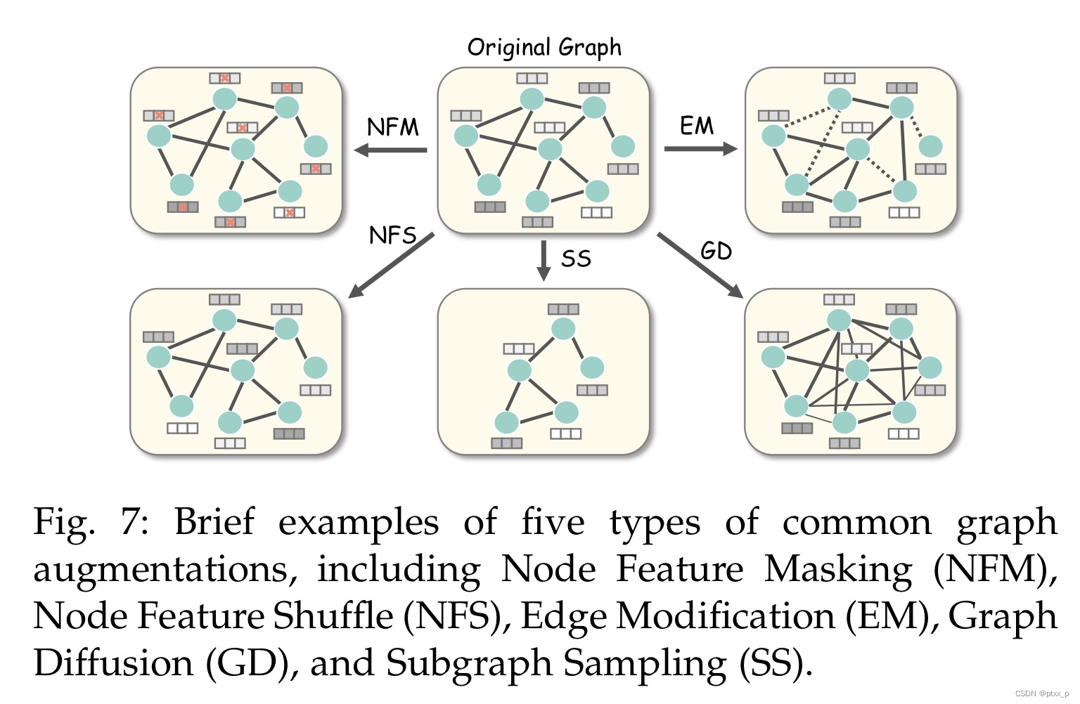
给定图$G$,the i-th augmented graph instance:${\tilde{G}}^{(i)}=t_i(G),t_i\sim \tau$ is a selected 图增强，$\tau$ is a set of available augmentations。

6.1.1 attributive augmentations

$G=(A,X)$, the augmented graph：
$${\tilde{G}}^{(i)}=(A,{\tilde{X}}^{(i)})=(A,t_i(X)).$$
attributive augmentations have 2 variants：node feature masking（NFM），node feature shuffle(NFS)。

node feature masking（NFM): 随机mask掉一部分节点的特征。
$$t_i(X)=M\circ X$$
M:masking matrix, $\circ$:哈达玛积。
除了M矩阵随机生成外，还可以calculate it adaptively：keep important nodes featires unmasked。

node feature shuffle(NFS): partially and row- wisely perturbs the node feature matrix。
$$t_i(X)=[X{]}_{\tilde{V}}.$$
$[\cdot {]}_{v_i}$: picking function that indexs the feature vector of $v_i$. $\tilde{V}$: partially shuffled node set。

6.1.2 topological augmentations

$${\tilde{G}}^{(i)}=({\tilde{A}}^{(i)},X)=(t_i(A),X).$$
两种典型方法是：edge modification(EM)、graph diffusion(GD).
edge modification(EM): 通过随机丢弃或者插入边来干扰给定的图邻接矩阵。
$$t_i(A)=M_1\circ A+M_2\circ (1-A).$$
$M_1,M_2$分别是edge dropping 和 insertion matrix，其实就是随机masking矩阵，它们也可以calculate adaptively。

graph diffusion(GD)： 为给定的邻接矩阵添加更加全局的拓扑信息：通过连接不直接连接的邻居。
$$t_i(A)=\sum _{k=0}^{\infty }{\Theta }_k{T}^k.$$
$\Theta$: weighting coefficient.
$T$: transition matrix.
特别的，具有两种初始化方法：

1. ${\Theta }_k=\frac{e^{-\iota }{t}^k}{k!},T=A{D}^{-1}.$
   $$t_i(A)=\exp (\iota A{D}^{-1}-\iota ).$$
   $\iota$: the diffusion time。

2. the personalized pagerank-based graph diffusion：
   ${\Theta }_k=\beta (1-\beta {)}^k,T=D^{-\frac{1}{2}}A{D}^{-\frac{1}{2}}.$
   $$t_i(A)=\beta (I-(1-\beta ))D^{-\frac{1}{2}}A{D}^{-\frac{1}{2}}.$$
   $\beta$: the tunable teleport probability.

6.1.3 hybrid augmentations

$${\tilde{G}}^{(i)}=({\tilde{A}}^{(i)},{\tilde{X}}^{(i)})=(t_i(A,X)).$$
一种典型的hybrid graph augmentation：subgraph sampling（SS）.
$$t_i(A,X)=[(A,X){]}_{V^{\prime }\in V}.$$
$V^{\prime }$是$V$的子集,可以使用多种的子集生成方法。
hybrid augmentations也可以是组合前面提到的多种图增强方法。

6.2 graph contrastive learning

可以大致分为：same-scale 、cross-scale contrastive learning。

6.2.1 same-scale contrast

可以进一步被分为：node-level和graph-level。

6.2.1.1 node-level same-scale contrast

$${\theta }^{\ast }=argmi{n}_{\theta }\frac{1}{|V|}\sum _{v_i\in V}{L}_{con}(p([f_{\theta }(A,X){]}_{v_i},[f_{\theta }(A,X){]}_{v_c})).$$
$v_c$: the contextual node of $v_i$, e.g. a neighboring node in a random walk starting from $v_i$.
这里的$p$一般是点乘。

modern node-level same-scale contrastive methods：under various graph augmentations, instead limiting on subgraph sampling.
$${\theta }^{\ast },{\varphi }^{\ast }=argmi{n}_{\theta ,\varphi }{L}_{con}(p_{\varphi }(f_{\theta }({\tilde{A}}^{(1)},{\tilde{X}}^{(1)}),f_{\theta }({\tilde{A}}^{(2)},{\tilde{X}}^{(2)}))).$$
拉近相似节点、推远不相关节点（构造负样本）。

6.2.1.2 graph-level same-scale contrast

$${\theta }^{\ast },{\varphi }^{\ast }=argmi{n}_{\theta ,\varphi }{L}_{con}(p_{\varphi }({\tilde{g}}^{(1)},{\tilde{g}}^{(2)})).$$
${\tilde{g}}^{(i)}=R(f_{\theta }({\tilde{A}}^{(i)},{\tilde{X}}^{(i)}))$, R is the readout function.

6.2.2 cross-scale contrast

可以大致被分为：patch-global and context- global contrast。

6.2.2.1 patch-global cross-scale contrast

$${\theta }^{\ast },{\varphi }^{\ast }=argmi{n}_{\theta ,\varphi }\frac{1}{|V|}\sum _{v_i\in V}{L}_{con}(p_{\varphi }([f_{\theta }(A,X){]}_{v_i},R(f_{\theta }(A,X)))).$$
node-level representation <-> graph-level representation：最大化它们之间的互信息，来帮助graph encoder to learn both localized and global semantic information。

上面提到的方法没有显式地使用图增强，使用图增强：
$${\theta }^{\ast },{\varphi }^{\ast }=argmi{n}_{\theta ,\varphi }\frac{1}{|V|}\sum _{v_i\in V}{L}_{con}(p_{\varphi }({\tilde{h}}_i^{(1)},{\tilde{g}}^{(2)})).$$
${\tilde{h}}_i^{(1)}=[f_{\theta }({\tilde{A}}^{(1)},{\tilde{X}}^{(1)}){]}_{v_i}$：representation of node $v_i$ in augmentation view1.
${\tilde{g}}^{(2)}=R(f_{\theta }({\tilde{A}}^{(2)},{\tilde{X}}^{(2)}))$：representation of augmentation view2.

6.2.2.2 context-global cross-scale contrast

context：上下文。
$${\theta }^{\ast },{\varphi }^{\ast }=argmi{n}_{\theta ,\varphi }\frac{1}{|S|}\sum _{s\in S}{L}_{con}(p_{\varphi }({\tilde{h}}_s,\tilde{g})).$$
$S$: 增强的输入图$\tilde{G}$的上下文子图集合(contextual subgraphs)，这里的图增强一般是图采样。
${\tilde{h}}_s$: the representation of augmented contextual subgraph s.
$\tilde{g}$: the graph-level representation over all subgraphs in S.

${\tilde{h}}_s=R([f_{\theta }(\tilde{A},\tilde{X}){]}_{v_i\in s}),\tilde{g}=R(f_{\theta }(\tilde{A},\tilde{X})).$

6.3 mutual information estimation

给定a pair of instance $(x_i,x_j)$, let $(h_i,h_j)$ denote their representations. the MI between $(i,j)$:

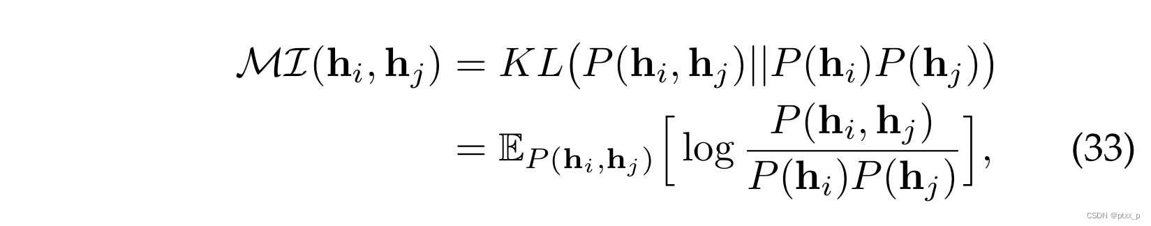
2 common forms of lower bound：Jensen-Shannon Estimator、Noise-Contrastive Estimator.

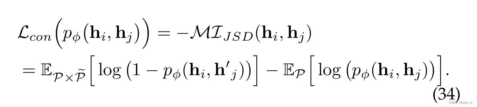
6.3.1 Jensen-Shannon Estimator

Jensen-Shannon (JSD): 提供了MI的有效估计和紧下界。基于JSD的对比损失定义如下：

$h_i,h_j\sim P,{\tilde{h}}_j^{\prime }\sim \tilde{P}$。
$p_{\varphi }(\cdot )$可以是多种形式：如bilinear transformation. $p_{\varphi }(h_i,h_j)=h_i^T\Phi h_j$…

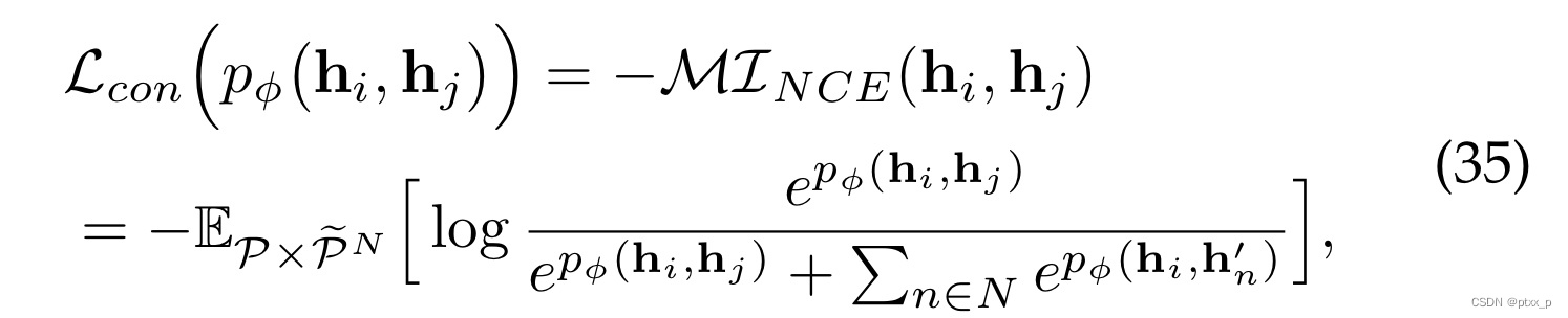
6.3.2 Noise-Contrastive Estimator

Noise-Contrastive Estimator也提供了a lower bound MI estimation，自然地关联了a positive and N negative pairs:

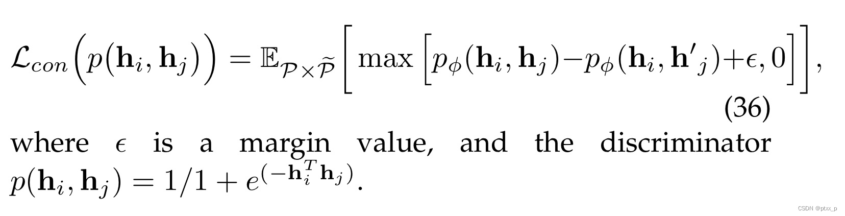
6.3.3 triplet loss

注意：minimizing this loss can not guarantee that the MI is being maximized because it cannot represent the lower bound of MI:

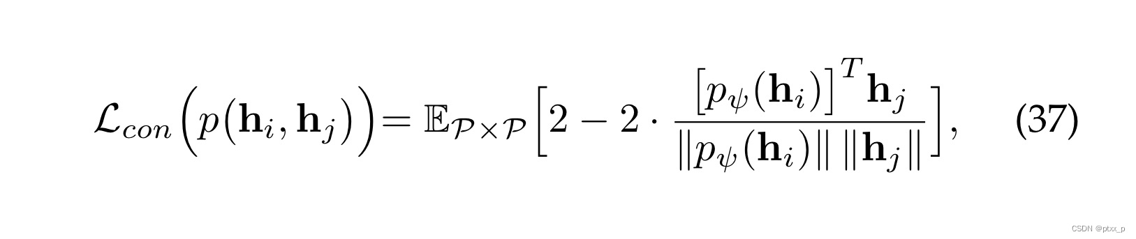
6.3.4 BYOL loss

not relying on negative samples：

6.3.5 Barlow Twins Loss

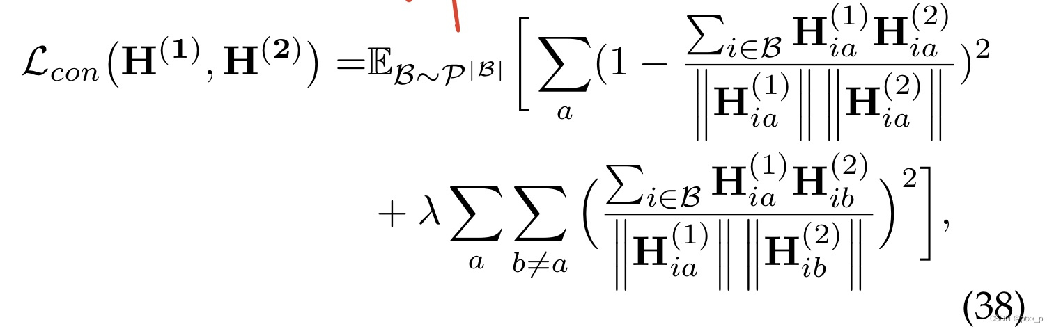
the representation of 2 views: $H^{(1)},H^{(2)}$ for a batch of data instances sampled from a distribution $P$.