TI mmWave radar sensors Tutorial 笔记 | Module 2: The phase of the IF signal

本系列为TI(Texas Instruments) mmWave radar sensors 系列视频公开课 的学习笔记。

• 视频网址: https://training.ti.com/intro-mmwave-sensing-fmcw-radars-module-1-range-estimation?context=1128486-1139153-1128542

• 关注 下面的公众号，回复“ TI毫米波 ”，即可获取 本系列完整的pdf笔记文件~

---

内容在CSDN和微信公众号同步更新

• CSDN博客
• 微信公众号

• Markdown源文件暂未开源
• 笔记难免存在问题，欢迎联系指正

FMCW Radars – Module 1 : Range Estimation
FMCW Radars – Module 2 : The Phase of the IF Signal
FMCW Radars – Module 3 : Velocity Estimation
FMCW Radars – Module 4 : Some System Design Topics
FMCW Radars – Module 5 : Angle Estimation

---

Module 2: The Phase of the IF Signal

Last Module: the frequency of IF signal

• $f_{IF}=S2d/c$

This Module:

• look into the phase of the IF signal
• The Phase is very important if we wish to understand the capability of FMCW radar to：

1. respond to very small displacements displacements 位移 in objects

2. measure the velocity very quickly and accurately

• 是heartbeat monitoring and vibration detection的基础

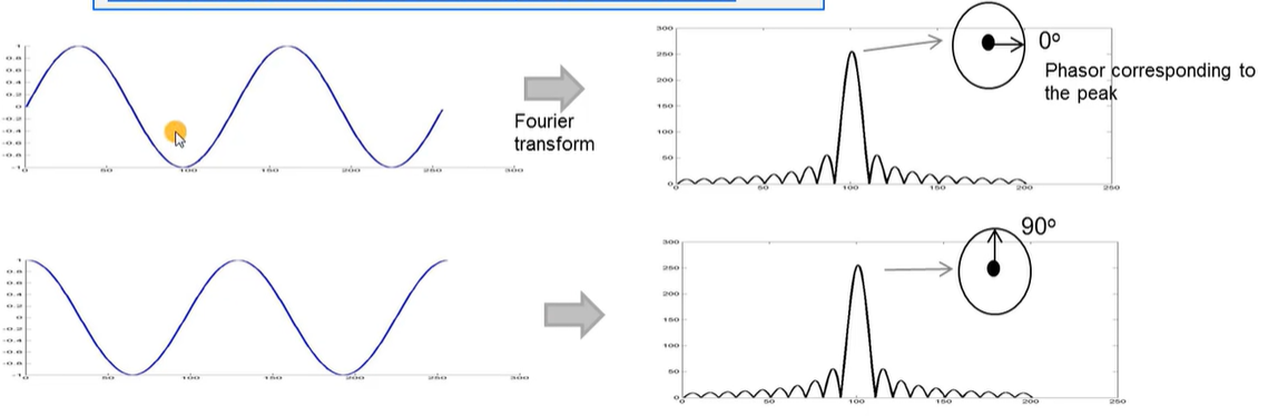
Fourier Transforms: A quick review

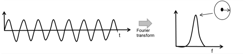
• Fourier Transform converts a time domain signal into the frequency domain
• A sinusoid in the time domain produces a peak in the frequency domain
• The signal in the Frequency domian is complex
  • each value is a phasor with a amplitude and a phase: $A{e}^{j\theta }$
  • 可用图形表示(如下图)

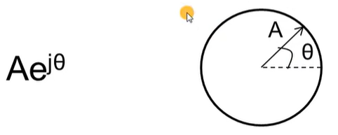
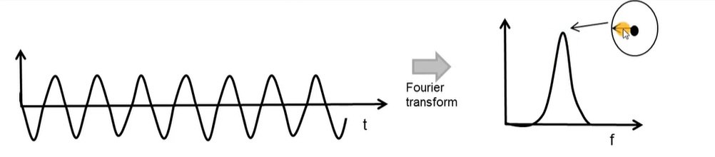
• Phase of the peak is equal to the initial phase of the sinusoid

Note: The above is strictly true only for a complex input tone (in the form of $e^{j\omega t}$)

• 但对于real input概念上也equally applicable with a few mathematical modifications
• 此处为了从概念上进行理解，忽略这些修正

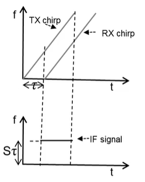
Frequency of the IF signal: Recap from module 1

• 两种观察方式：
  • A-t plot
  • f-t plot
• In module 1, focus on f-t plot to understand the IF signal
  • A single object in front of the radar produces an IF signal with a constant frequency of $S2d/c$

• This module:
  • use the A-t plot to analyze the relationship between the Phase and the Distance

Phase of the IF signal

• Let’s look at the ‘A-t’ plot

  • To get more intuition into the nature of the IF signal

• IF signal:

  • For an object at a distance d from the radar, the IF signal will be a sinusoid:

  • $Asin(2\pi ft+{\varphi }_0)$

  • 其中$f=S2d/c$

  • What is the ${\varphi }_0$ :

    🚩 The phase of point C in the following image C点相位

    🚩 Recall: mixer输出信号的initial phase就是 the difference of the initial phase of the two inputs $\Rightarrow$ 即 (A点相位 - B点相位)

    🚩 也是 the peak point in FFT(IF signal) 的相位

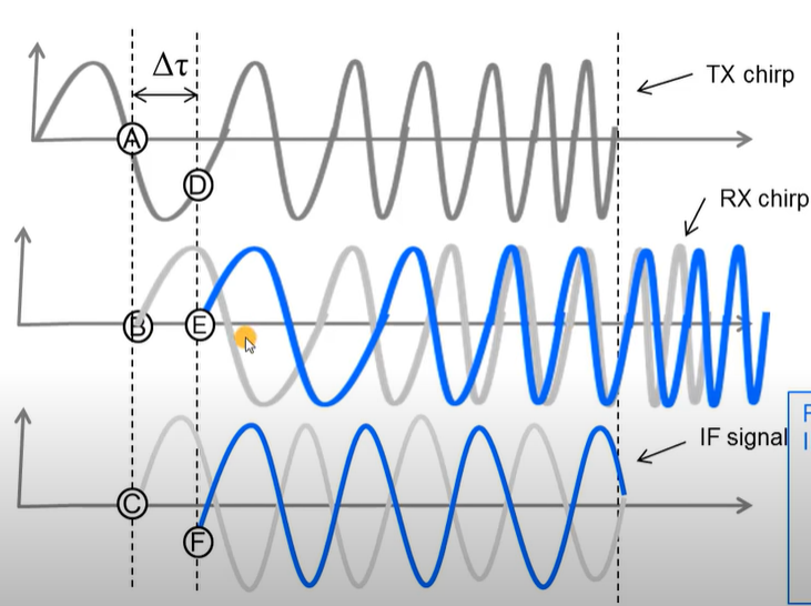
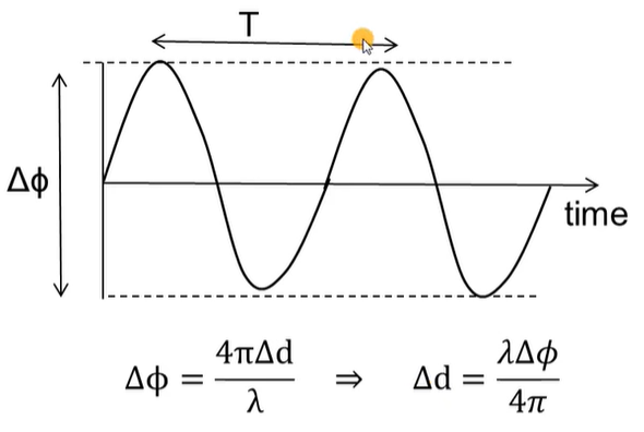
• 相移 VS 位移 ：what happens to the phase fo the IF signal if the object moves by a small ditance $\Delta \tau$?

  • 灰色曲线: before the movement

  • 蓝色曲线: after the movement

  • The phase of the TX: delay

    🚩 Phase diference between A and D: $\Delta \Phi =2\pi f_c\Delta \tau =\frac{4\pi \Delta d}{\lambda }$

  • The phase of the RX: 不变 (注: 因为根据电磁场与波，垂直入射相位改变$\pi$, 所以不变)

  • Therefore, $\Delta \varphi$ of IF signal = $\Delta \varphi$ of TX signal $=\Delta \Phi =2\pi f_c\Delta \tau =\frac{4\pi \Delta d}{\lambda }$

  • 最终结论: $\frac{4\pi \Delta d}{\lambda }$

Sensitivity of the IF signal for small displacements in the object

• Recall: the IF signal is $Asin(2\pi ft+{\varphi }_0)$

  • $f=S2d/c$
  • $\Delta \varphi =\frac{4\pi \Delta d}{\lambda }$

• Now: 如果目标物体位移了一小段，IF signal的频率和相位将会如何变化？

  • 一小段(small): compared to the range resolution of the radar

---

• An example:

  • $S=50MHz/us$, $T_c=40us$, $77GHz$, $1mm=\lambda /4$

  • What happens if an object in front of the randar changes its position by $1mm$

  • Phase: $\Delta \varphi =\frac{4\pi \Delta d}{\lambda }=\pi =180^{\circ }$

  • Frequency: by $\Delta \mathrm{f}=\frac{\mathrm{S}2\Delta d}{c}=\frac{50\times 10^{12}\times 2\times 1\times 10^{-3}}{3\times 10^8}=333\mathrm{Hz}$

    🚩 但 尽管 333 Hz looks like a big number $\Rightarrow$ But in the observation window , this corresponds to only additional $\Delta f{T}_c=333\times 40\times 10^{-6}=0.013$ cycles

    ❌ $\Rightarrow$ 在频谱图中不会被体现

---

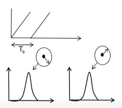
结论 : The phase of the IF signal is very sensitive to small changes in object range.

• 如下图所示
  • An object at certain distance produces an IF signal with a certain frequency and phase (上图)
  • small motion in the object changes the phase of the IF signal but not the frequency

How to measure the velocity (v) of an object using 2 chirps?

• Transmit two chirps separated by $T_c$
• The range-FFTs corresponding to each chirp will have peaks in the same location but with different phase
• The measured phase difference $\omega$ corresponds to a motion in the object of $v{T}_c$
  • $\omega =\frac{4\pi v{T}_c}{\lambda }$
  • $\Rightarrow$ $v=\frac{\lambda \omega }{4\pi T_c}$

结论 : The phase difference measured across two consecutive chirps can be used to estimate the velocity of the object

Measurements on a Vibrating Object

• blue block:
  • Small (amplitude ~1mm) vibrations over time
  • $\Delta d$ is a fraction of a wavelength

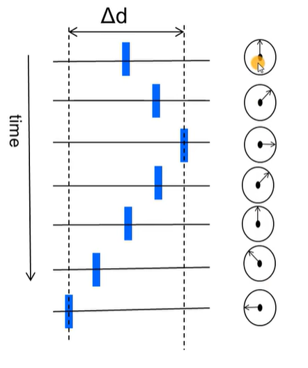
• measure the time evolution of phase
  • obtained by FFT
  • can be used to estimate both the amplitude and periodicity of the vibration

Epilogue

• What we learned in this module:

  • The phase of IF signal is very sensitve to small changes in the range of the object
  • we can exploit it to meaure the velocity
  • $\Delta \varphi =\frac{4\pi \Delta d}{\lambda }$
  • $v=\frac{\lambda \Delta \varphi }{4\pi T_c}$

• 下一个目标：

  • How to separate Multiple objects equidistant from the radar, but with differing velocities relative to the radar

    🚩 Equi-range objects which have differing velocities relative to the radar can be separated out using a “Doppler-FFT”

    ✅ see in the next module