通过氨基酸频率特征量来预测蛋白热稳定性——随机森林算法

一、随机森林算法原理

随机森林算法生成过程：

1、从原始数据集中每次随机有放回抽样选取与原始数据集相同数量的样本数据，构造数据子集；

2、每个数据子集从所有待选择的特征中随机选取一定数量的最优特征作为决策树的输入特征；

3、根据每个数据子集分别得到每棵决策树，由多棵决策树共同组成随机森林；

4、最后如果是分类问题，则按照投票的方式选取票数最多的类作为结果返回，如果是回归问题，则按照平均法选取所有决策树预测的平均值作为结果返回。

二、构建我们要分析的数据集

    这里以我研究的领域——裂解酶为例，裂解酶作为一种噬菌体（细菌病毒）来源的水解酶，其可以在体外快速裂解细菌细胞壁肽聚糖，造成细菌裂解死亡。随着细菌耐药问题日益突出，裂解酶有望成为后抗生素时代的抗菌候选药物。然而裂解酶作为蛋白质类抗菌剂，其热稳定性是制约其发展成为一种物美价廉药物的瓶颈。

      通常未经过表达系统修饰的蛋白，其一级结构决定了其三级结构，而结构又决定其功能，蛋白的一级结构由20种氨基酸组成，因此氨基酸组成有可能成为区分裂解酶热稳定性的重要特征。为回答这一问题，我们通过数据库找到噬热噬菌体蛋白序列，以及热稳定性一般的水解酶类蛋白序列，然后统计蛋白的氨基酸频率，之后通过机器学习——随机森林，把蛋白氨基酸频率作为特征量让机器去学习、训练，并预测蛋白质的热稳定性。这里序列就不展示了。

1）将噬热噬菌体蛋白序列读取，序列列表记住为lysin_b​​​​​​

lysin = ''
a = ""
f = open("/home/lxh/Documents/python实战算法/裂解酶热稳定_随机森林/Thermus_thermophilus_phage_protein.txt","r")
for line in f.readlines():
  a = line.replace('\n','')
  lysin += a

b = lysin.split('>')
lysin_b = []
del b[0]
for line in b:
  if line.find('[gbkey=CDS]') != -1:
    aa = line[line.index('[gbkey=CDS]') + 11:]
    if aa not in lysin_b:
      lysin_b.append(aa)

2）同理将常温酶读取，代码不展示......,序列列表记住为lysin_k

3）为了获取可能有活性的蛋白，我们对蛋白长度进行了限制

def lysin_jiequ(lysin):
  global lysino
  lysino = []
  for i in lysin:
    if (len(i) < 300) & (len(i) > 100):
      lysino.append(i)

      运行将上述函数后，直接调用lysin_jiequ(),括号内输入我们的两种类型的蛋白列表进行截取长度在100-300aa的蛋白，通过len()函数我们查阅到截取前后lysin_b分别为10324条、4928条，lysin_k分别为600条、434条。为了减少后面计算误差，我们选择lysin_b截取后的前500条序列作为噬热蛋白序列集合。

3）统计每条蛋白序列中20种氨基酸的频率

def aa_freq(lysin_b):
  import numpy
  import numpy as np
  global sum2
  sum1 = []
  sum2 = []
  a = ['G','A','V','L','I','F','P','S','T','H','W','C','D','E','K','Y','M','N','Q','R']
  for x in lysin_b:
    for y in a:
      sum = format(x.count(y)/len(x),'.3f')
      sum1.append(float(sum))
    sum2.append(sum1)  
    sum1 = []

   将截取后的lysin_b和lysin_k序列合并，运行上述函数后，调用此函数统计蛋白氨基酸频率。

4）添加区分噬热酶和常温的标签

i = 0
for a in sum2:
  i += 1
  if i < 501:
    a.append(1)
  else:
    a.append(2)

    标签为thermo，噬热酶标签值为1，有500条序列，常温酶标签为2，有434条序列。将1或者2加入到每条序列的最后一位。

5）将sum2列表转化为矩阵

#将sum2转化为矩阵
import numpy as np
sum2_mat = np.array(sum2)

    运行sum2_mat.shape，我们可以看到sum2_mat形成了934行，21列的矩阵。

>>> sum2_matarray([[ 0.08,  0.07,  0.06, ...,  0.03,  0.09,  1.  ],       [ 0.03,  0.01,  0.06, ...,  0.01,  0.04,  1.  ],       [ 0.07,  0.02,  0.06, ...,  0.01,  0.03,  1.  ],       ...,        [ 0.13,  0.09,  0.08, ...,  0.02,  0.04,  2.  ],       [ 0.11,  0.09,  0.1 , ...,  0.03,  0.04,  2.  ],       [ 0.14,  0.09,  0.05, ...,  0.03,  0.06,  2.  ]])>>> sum2_mat.shape(934, 21)

        每一行代表一条蛋白序列，20列分别表示20种氨基酸，其中的数值表示氨基酸频率。最后一列表示热稳定标签。

4）将矩阵数据保存到本地，方便下次直接读取

import csv
import pandas as pd
aa = ['G','A','V','L','I','F','P','S','T','H','W','C','D','E','K','Y','M','N','Q','R','thermo']
pd.DataFrame(sum2,columns = aa).to_csv('/home/lxh/Documents/python实战算法/裂解酶热稳定_随机森林/lysin_aa_freq.csv')

三、机器学习、训练、预测——随机森林法

1）数据读取,并进行数据的检查

import pandas as pd
# Read in data and display first 5 rows
features = pd.read_csv('/home/lxh/Documents/python实战算法/裂解酶热稳定_随机森林/lysin_aa_freq.csv')
features = features.iloc[:,1:]#删除第一列的索引值
features.head(5)
features.info()
features.shape
features.describe()

2)数据预处理，单热点编码

features = pd.get_dummies(features)#可将数据中的有序文字转化为可读取的数字型
features.iloc[:,5:].head(5)#读取第5列以后的数据查验

     本文数据类型为float，可忽略这一步。

3）对单个特征量进行相关性分析

    直方图

import seaborn as sns
import matplotlib.pyplot as plt
%matplotlib inline
plt.figure(figsize=(8,4))
sns.barplot(x='G',y='thermo',data=features)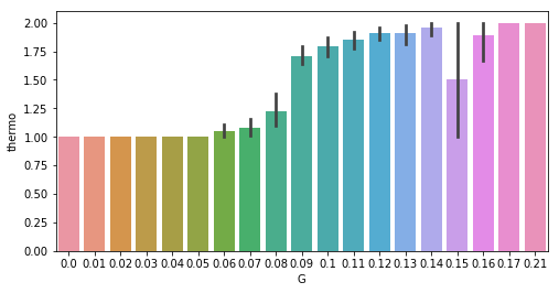

4） 分离特征量和标签

# Use numpy to convert to arrays
import numpy as np
# Labels are the values we want to predict
labels = np.array(features['thermo'])
# Remove the labels from the features
# axis 1 refers to the columns
features= features.drop('thermo', axis = 1)
# Saving feature names for later use
feature_list = list(features.columns)
# Convert to numpy array
features = np.array(features)

5)将数据分为训练集和测试集

# Using Skicit-learn to split data into training and testing sets
from sklearn.model_selection import train_test_split
# Split the data into training and testing sets
train_features, test_features, train_labels, test_labels = train_test_split(features, labels, test_size = 0.25, random_state = 42)

     test_size=0.25表示随机抽取1/4的数据作为测试集

6）开始机器学习训练

# Import the model we are using
from sklearn.ensemble import RandomForestRegressor
# Instantiate model with 1000 decision trees
rf = RandomForestRegressor(n_estimators = 1000, random_state = 42)
# Train the model on training data
rf.fit(train_features, train_labels);

7）测试集预测结果并计算正确率

# Use the forest's predict method on the test data
predictions = rf.predict(test_features)
# Calculate the absolute errors
errors = abs(predictions - test_labels)
mape = 100 * (errors / test_labels)
# Calculate and display accuracy
accuracy = 100 - np.mean(mape)
print('Accuracy:', round(accuracy, 2), '%.')

测试集蛋白序列有934*0.25=234条，准确率为95.4%，结果还不错！

8）训练好的模型用于实际样本预测

predictions = rf.predict(实际样本20种氨基酸矩阵)

    运行aa_freq(),后将其转化为矩阵，带入上述函数，运行predictions，可得到计算值，数值越接近1，表示热稳定性越好，越接近2表示热稳定越差。本次输入四条蛋白序列（记为A、B、C、D），实验证实其热稳定性排序为A>B，C>D，通过本次机器学习预测结果为A：1.865；B：1.868；C：1.805；D：1.855。

结果正确。

9）特征量重要性分析

     图表形式

importances = rf.feature_importances_
a = pd.DataFrame()
a['特征'] = feature_list
a['特征重要性'] = importances
a = a.sort_values('特征重要性',ascending=False)
a

   图片形式

importances = rf.feature_importances_
a = pd.DataFrame()
a['features'] = feature_list
a['importances'] = importances
a = a.sort_values('importances',ascending=False)

import seaborn as sns
import matplotlib.pyplot as plt
%matplotlib inline
sns.barplot(x='features',y='importances',data=a)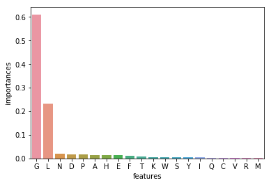

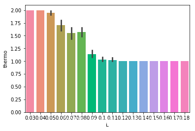
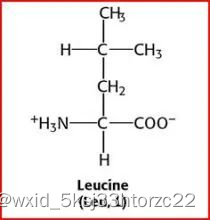
使用第3）步代码，将L也做相关性分析

四、结论与分析

1）结论

    甘氨酸和亮氨酸对于蛋白热稳定性贡献较大，热稳定性好的蛋白中亮氨酸含量较高，甘氨酸含量较少，热稳定差的蛋白中甘氨酸含量较高，亮氨酸含量较少。

2）分析 

      G（Gly）甘氨酸，为中性亲水氨基酸，L（Leu）亮氨酸，为疏水氨基酸，更易在蛋白疏水内核，起到稳定蛋白结构的作用。

可参考微信推文：通过特征量来预测蛋白热稳定性——随机森林算法