


理解深度学习的卷积层、激活层、池化层
网上看了些教程,感觉还是来点实例可能更好理解一些。
下面分别把卷积层nn.Conv2d()、激活层nn.ReLU()、池化层nn.MaxPool2d()用代码表示出来,并且用图片显示加以理解。
读取图片
先读取一张图片,用来做卷积等操作的示范。
用cv2来读取读片,并转换成深度学习网络可使用的数据格式。
因为神经网络中有一个batch size的功能,但我们只有一张图片,所以需要image.unsqueeze(0) 一下增加一个数量
# 将图片转换为模型可用的数据
def getImageData(imgFile):
    image = cv2.imread(imgFile, 0)
    image = F.to_tensor(image)  # shape为 [1, 768, 1024], [通道,高,宽]
    image = image.unsqueeze(0)  # shape为 [1, 1, 768, 1024], [数量,通道,高,宽]
    return image
显示图片
在图片做完卷积、激活、池化后,需要将图片显示出来,用来观察这些操作到底做了什么事情。
显示图片,用的是matplotlib.pyplot。
这里只显示三个图片做示例。
# 将三个图片显示在plt上
def showTensorImg(image, title=""):
    plt.figure(title)  # 创建第一个图形
    plt.sca(plt.subplot(1, 3, 1))  # 分成1行2列,选择第1个位置
    plt.imshow(image[0].data, cmap=plt.cm.gray)
    plt.sca(plt.subplot(1, 3, 2))  # 分成1行2列,选择第2个位置
    plt.imshow(image[1].data, cmap=plt.cm.gray)
    plt.sca(plt.subplot(1, 3, 3))  # 分成1行2列,选择第2个位置
    plt.imshow(image[2].data, cmap=plt.cm.gray)
定义一个神经网络
用一个神经网络,在其中加入卷积层。
这里构建网络,用的是pytorch的 torch.nn。
# 定义模型
class MyModel(nn.Module):
    def __init__(self):
        super(MyModel, self).__init__()
        self.conv0 = nn.Conv2d(in_channels=1, out_channels=3, kernel_size=(3, 3), stride=1, padding=1)

    # 把模型里的卷积层和激活层后的效果,显示出来看一看
    def forward(self, image):
        img = self.conv0(image)
        print("conv0:", img, img.shape, "\n")
        showTensorImg(img.squeeze(), "conv0")

        return img
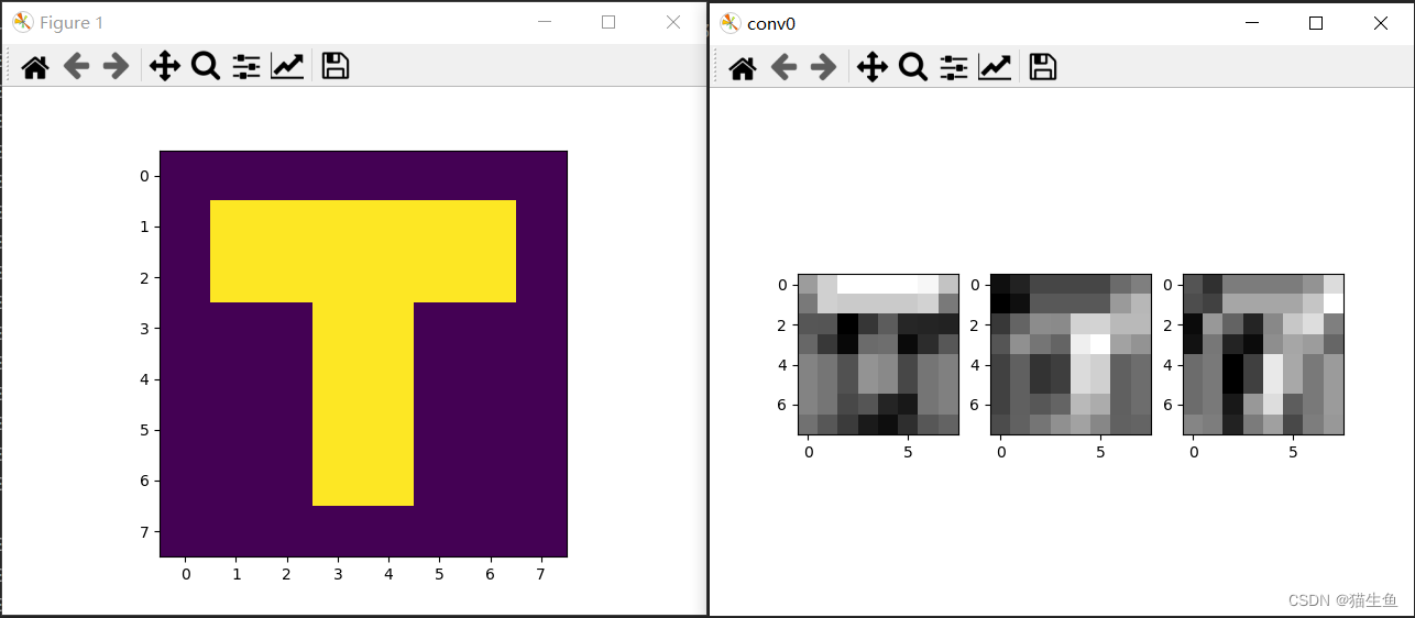
查看卷积层结果
拿一张图片来做示范,先显示原图,再显示卷积层的结果。
if __name__ == "__main__":
    # 显示原图
    img = cv2.imread("Data/2.jpeg", 0)
    plt.imshow(img)
    print(img.shape)

    net = MyModel()
    image = getImageData("Data/2.jpeg")
    img = net(image)

    plt.show()
看看显示结果:
看看输出结果:
(8, 8)
conv0: tensor([[[[ 0.4108,  0.6527,  0.8689,  0.8689,  0.8689,  0.8689,  0.8303, 0.5918],
          [ 0.2540,  0.6494,  0.6211,  0.6211,  0.6211,  0.6211,  0.6613, 0.2530],
          [ 0.0873,  0.0837, -0.3083, -0.0584,  0.1192, -0.1307, -0.1400, -0.1493],
          [ 0.1661, -0.0434, -0.2697,  0.1860,  0.1980, -0.2577, -0.1014, 0.0951],
          [ 0.2942,  0.2339,  0.0656,  0.3721,  0.3261,  0.0195,  0.2339, 0.2812],
          [ 0.2942,  0.2339,  0.0656,  0.3721,  0.3261,  0.0195,  0.2339, 0.2812],
          [ 0.2942,  0.2339,  0.0270,  0.0837, -0.1400, -0.1967,  0.2339, 0.2812],
          [ 0.2130,  0.0919, -0.0362, -0.1854, -0.2434, -0.0942,  0.0919, 0.1501]],

         [[-0.4264, -0.3058, -0.0771, -0.0771, -0.0771, -0.0771,  0.1542, 0.2827],
          [-0.5278, -0.4299,  0.0381,  0.0381,  0.0381,  0.0381,  0.4555, 0.6393],
          [-0.1677,  0.1134,  0.3660,  0.3549,  0.8149,  0.8260,  0.6546, 0.6552],
          [ 0.0183,  0.3910,  0.2182,  0.1155,  1.0009,  1.1036,  0.5068, 0.4159],
          [-0.1105,  0.0901, -0.1985, -0.1290,  0.8722,  0.8027,  0.0901, 0.1713],
          [-0.1105,  0.0901, -0.1985, -0.1290,  0.8722,  0.8027,  0.0901, 0.1713],
          [-0.1105,  0.0901,  0.0328,  0.1134,  0.6546,  0.5740,  0.0901, 0.1713],
          [-0.0422,  0.0939,  0.2227,  0.3948,  0.5107,  0.3385,  0.0939, 0.1101]],

         [[-0.0304, -0.1294,  0.0825,  0.0825,  0.0825,  0.0825,  0.1528, 0.3564],
          [-0.0499, -0.0802,  0.2031,  0.2031,  0.2031,  0.2031,  0.2914, 0.4559],
          [-0.2361,  0.1632,  0.0132, -0.1656,  0.1166,  0.2954,  0.3580, 0.0929],
          [-0.2182,  0.0699, -0.1696, -0.2371,  0.1346,  0.2021,  0.1752, 0.0214],
          [ 0.0384,  0.0756, -0.2692, -0.0859,  0.3911,  0.2077,  0.0756, 0.1726],
          [ 0.0384,  0.0756, -0.2692, -0.0859,  0.3911,  0.2077,  0.0756, 0.1726],
          [ 0.0384,  0.0756, -0.1989,  0.1632,  0.3580, -0.0041,  0.0756, 0.1726],
          [ 0.1085,  0.0860, -0.1705,  0.0804,  0.1857, -0.0651,  0.0860, 0.1633]]]],
      grad_fn=<ThnnConv2DBackward0>) torch.Size([1, 3, 8, 8])
我的输入是图片的灰度单通道,但经过卷积后可以输出3通道甚至更多。
再看输出的shape,图片宽高均为(8,8),没有改变。
卷积的原理:

(图片我是从这里搬过来的,感谢作者!)
卷积核为(3,3),每(3,3)的方块中通过卷积运算得到一个像素值。因为在卷积时使用了一个padding=1,所以在原图四周多出一个像素,也就导致卷积图和原图保持同一个大小。
卷积的原理看这儿。
神经网络中添加一个激活层
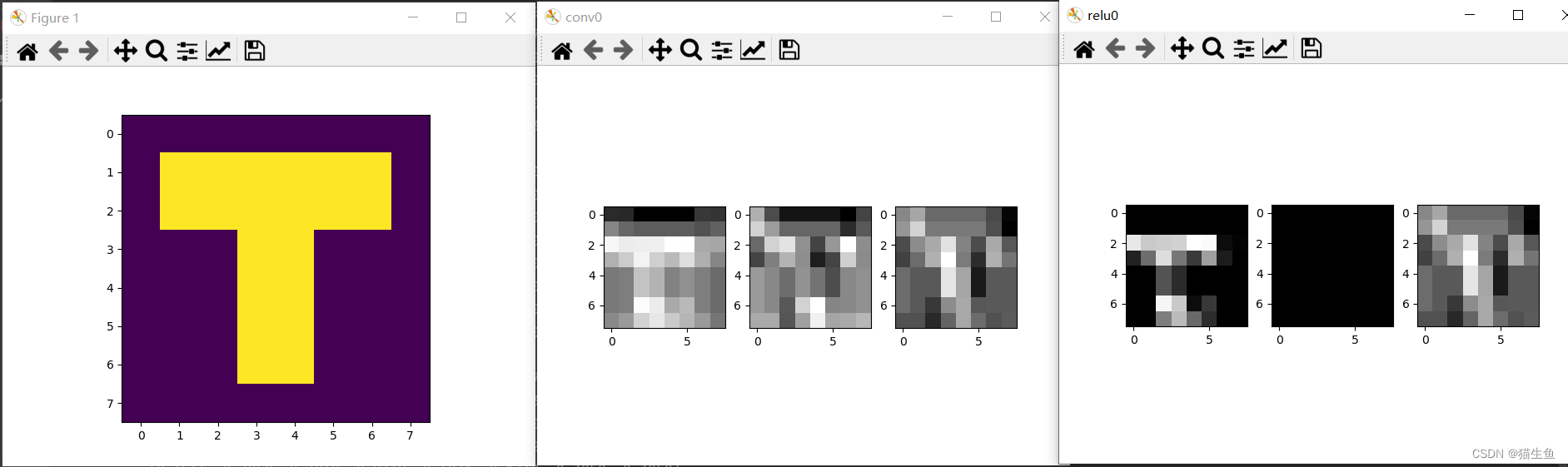
这里使用的激活函数为nn.ReLU(),先添加运行看看结果。
# 定义模型
class MyModel(nn.Module):
    def __init__(self):
        super(MyModel, self).__init__()
        self.conv0 = nn.Conv2d(in_channels=1, out_channels=3, kernel_size=(3, 3), stride=1, padding=1)
        self.relu0 = nn.ReLU(inplace=True)

    # 把模型里的卷积层和激活层后的效果,显示出来看一看
    def forward(self, image):
        img = self.conv0(image)
        print("conv0:", img, img.shape, "\n")
        showTensorImg(img.squeeze(), "conv0")

        img = self.relu0(img)
        print("relu0:", img, img.shape, "\n")
        showTensorImg(img.squeeze(), "relu0")

        return img
再看看输出结果:
(8, 8)
conv0: tensor([[[[-0.4327, -0.4364, -0.5815, -0.5815, -0.5815, -0.5815, -0.3790, -0.3967],
          [-0.1099, -0.2190, -0.2511, -0.2511, -0.2511, -0.2511, -0.2947, -0.2357],
          [ 0.2893,  0.2509,  0.2563,  0.2617,  0.3190,  0.3136,  0.0159, 0.0043],
          [ 0.0433,  0.1370,  0.2754,  0.1487,  0.0730,  0.1997,  0.0351, -0.1086],
          [-0.1535, -0.1358,  0.1045,  0.0538, -0.1238, -0.0732, -0.1358, -0.2035],
          [-0.1535, -0.1358,  0.1045,  0.0538, -0.1238, -0.0732, -0.1358, -0.2035],
          [-0.1535, -0.1358,  0.3070,  0.2509,  0.0159,  0.0720, -0.1358, -0.2035],
          [-0.0980, -0.0395,  0.1572,  0.2333,  0.1314,  0.0553, -0.0395, -0.1642]],

         [[-0.2516, -0.4649, -0.5853, -0.5853, -0.5853, -0.5853, -0.6295, -0.4837],
          [-0.1780, -0.2942, -0.4109, -0.4109, -0.4109, -0.4109, -0.5343, -0.4370],
          [-0.4042, -0.1781, -0.1395, -0.3199, -0.4845, -0.3040, -0.0809, -0.3259],
          [-0.4835, -0.3571, -0.2429, -0.3237, -0.5638, -0.4830, -0.1843, -0.3296],
          [-0.3014, -0.3369, -0.3955, -0.3145, -0.3818, -0.4628, -0.3369, -0.3204],
          [-0.3014, -0.3369, -0.3955, -0.3145, -0.3818, -0.4628, -0.3369, -0.3204],
          [-0.3014, -0.3369, -0.4396, -0.1781, -0.0809, -0.3423, -0.3369, -0.3204],
          [-0.2631, -0.2646, -0.4467, -0.2849, -0.1120, -0.2739, -0.2646, -0.2357]],

         [[ 0.5655,  0.6888,  0.4497,  0.4497,  0.4497,  0.4497,  0.3205, 0.0511],
          [ 0.6213,  0.8629,  0.5083,  0.5083,  0.5083,  0.5083,  0.3436, 0.0312],
          [ 0.3276,  0.5826,  0.6993,  0.9224,  0.5541,  0.3310,  0.6991, 0.3734],
          [ 0.2920,  0.4577,  0.7255,  1.0379,  0.5186,  0.2062,  0.7253, 0.4888],
          [ 0.4566,  0.3858,  0.3860,  0.9348,  0.6831,  0.1342,  0.3858, 0.3858],
          [ 0.4566,  0.3858,  0.3860,  0.9348,  0.6831,  0.1342,  0.3858, 0.3858],
          [ 0.4566,  0.3858,  0.2568,  0.5826,  0.6991,  0.3734,  0.3858, 0.3858],
          [ 0.3575,  0.3540,  0.1894,  0.4259,  0.6935,  0.4570,  0.3540, 0.3903]]]],
       grad_fn=<ThnnConv2DBackward0>) torch.Size([1, 3, 8, 8])

relu0: tensor([[[[0.0000, 0.0000, 0.0000, 0.0000, 0.0000, 0.0000, 0.0000, 0.0000],
          [0.0000, 0.0000, 0.0000, 0.0000, 0.0000, 0.0000, 0.0000, 0.0000],
          [0.2893, 0.2509, 0.2563, 0.2617, 0.3190, 0.3136, 0.0159, 0.0043],
          [0.0433, 0.1370, 0.2754, 0.1487, 0.0730, 0.1997, 0.0351, 0.0000],
          [0.0000, 0.0000, 0.1045, 0.0538, 0.0000, 0.0000, 0.0000, 0.0000],
          [0.0000, 0.0000, 0.1045, 0.0538, 0.0000, 0.0000, 0.0000, 0.0000],
          [0.0000, 0.0000, 0.3070, 0.2509, 0.0159, 0.0720, 0.0000, 0.0000],
          [0.0000, 0.0000, 0.1572, 0.2333, 0.1314, 0.0553, 0.0000, 0.0000]],

         [[0.0000, 0.0000, 0.0000, 0.0000, 0.0000, 0.0000, 0.0000, 0.0000],
          [0.0000, 0.0000, 0.0000, 0.0000, 0.0000, 0.0000, 0.0000, 0.0000],
          [0.0000, 0.0000, 0.0000, 0.0000, 0.0000, 0.0000, 0.0000, 0.0000],
          [0.0000, 0.0000, 0.0000, 0.0000, 0.0000, 0.0000, 0.0000, 0.0000],
          [0.0000, 0.0000, 0.0000, 0.0000, 0.0000, 0.0000, 0.0000, 0.0000],
          [0.0000, 0.0000, 0.0000, 0.0000, 0.0000, 0.0000, 0.0000, 0.0000],
          [0.0000, 0.0000, 0.0000, 0.0000, 0.0000, 0.0000, 0.0000, 0.0000],
          [0.0000, 0.0000, 0.0000, 0.0000, 0.0000, 0.0000, 0.0000, 0.0000]],

         [[0.5655, 0.6888, 0.4497, 0.4497, 0.4497, 0.4497, 0.3205, 0.0511],
          [0.6213, 0.8629, 0.5083, 0.5083, 0.5083, 0.5083, 0.3436, 0.0312],
          [0.3276, 0.5826, 0.6993, 0.9224, 0.5541, 0.3310, 0.6991, 0.3734],
          [0.2920, 0.4577, 0.7255, 1.0379, 0.5186, 0.2062, 0.7253, 0.4888],
          [0.4566, 0.3858, 0.3860, 0.9348, 0.6831, 0.1342, 0.3858, 0.3858],
          [0.4566, 0.3858, 0.3860, 0.9348, 0.6831, 0.1342, 0.3858, 0.3858],
          [0.4566, 0.3858, 0.2568, 0.5826, 0.6991, 0.3734, 0.3858, 0.3858],
          [0.3575, 0.3540, 0.1894, 0.4259, 0.6935, 0.4570, 0.3540, 0.3903]]]],
       grad_fn=<ReluBackward0>) torch.Size([1, 3, 8, 8])
从输出的结果可以看到,nn.ReLU()激活函数,将卷积的结果图片中,所有小于0的值被被置零了,并不会改变图片的大小。
因为值越大,特征就越是突出,那将小于0的值全部抹掉,可以减少模型的计算。
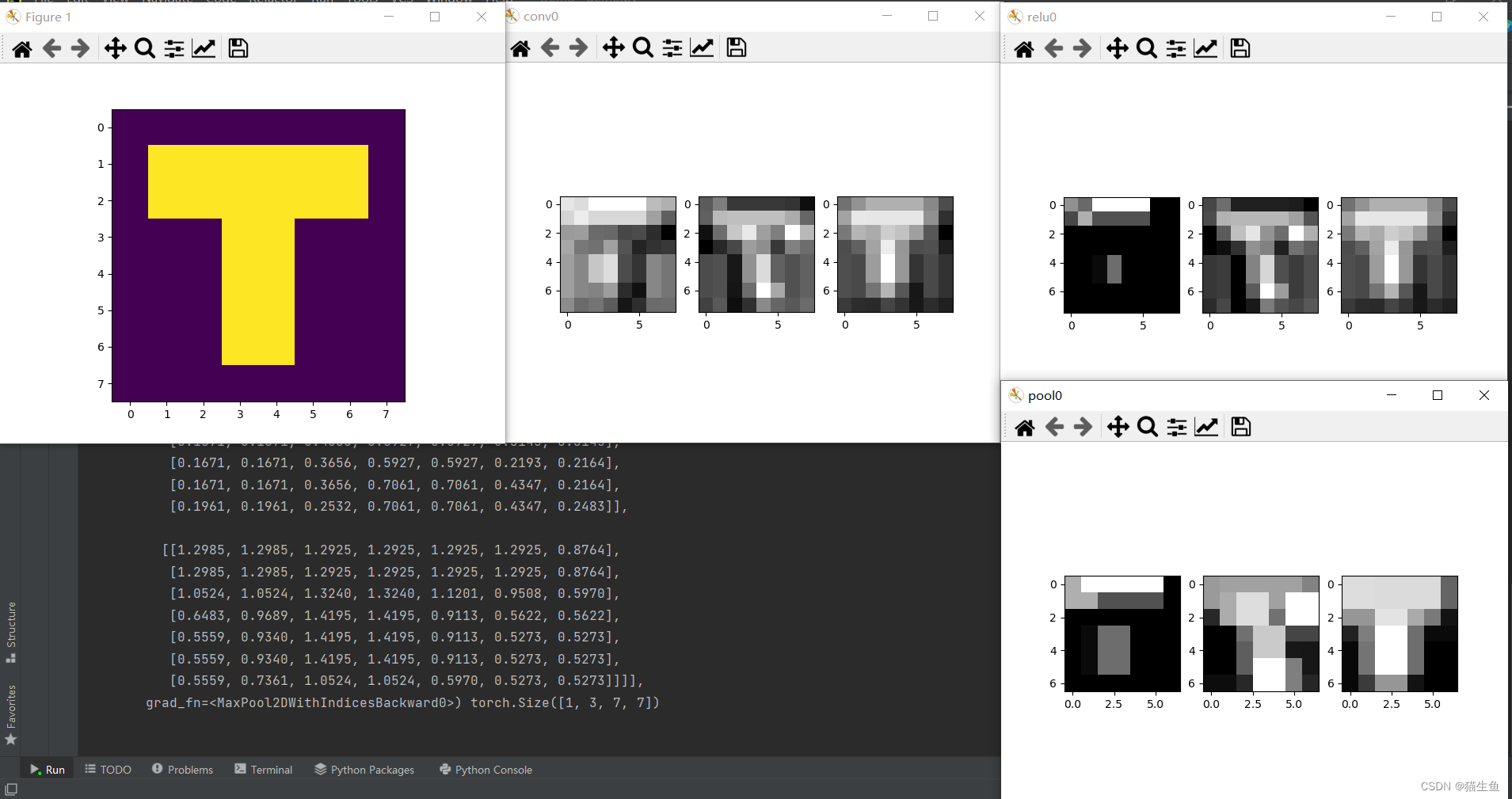
神经网络中添加一个池化层
这里池化层用的是最大池化,nn.MaxPool2d(),平均池化的话可以自己尝试一下。
# 定义模型
class MyModel(nn.Module):
    def __init__(self):
        super(MyModel, self).__init__()
        self.conv0 = nn.Conv2d(in_channels=1, out_channels=3, kernel_size=(3, 3), stride=1, padding=1)
        self.relu0 = nn.ReLU(inplace=True)
        self.pool0 = nn.MaxPool2d(kernel_size=2, stride=1)

    # 把模型里的卷积层和激活层后的效果,显示出来看一看
    def forward(self, image):
        img = self.conv0(image)
        print("conv0:", img, img.shape, "\n")
        showTensorImg(img.squeeze(), "conv0")

        img = self.relu0(img)
        print("relu0:", img, img.shape, "\n")
        showTensorImg(img.squeeze(), "relu0")

        img = self.pool0(img)
        print("pool0:", img, img.shape, "\n")
        showTensorImg(img.squeeze(), "pool0")

        return img
输出结果:
D:\ProgramData\anaconda3\envs\Python3.8.5-Pytorch\python.exe E:/work/Python/Demo/demo.py
(8, 8)
conv0: tensor([[[[ 0.1296,  0.0942,  0.2273,  0.2273,  0.2273,  0.2273, -0.0275, -0.0733],
          [ 0.0647,  0.1555,  0.0734,  0.0734,  0.0734,  0.0734, -0.1328, -0.3786],
          [-0.1575, -0.1451, -0.3350, -0.3473, -0.4690, -0.4568, -0.5740, -0.7413],
          [-0.1089, -0.2873, -0.3107, -0.1321, -0.4204, -0.5990, -0.5496, -0.5262],
          [-0.1416, -0.2293,  0.0097,  0.0975, -0.4531, -0.5410, -0.2293, -0.2965],
          [-0.1416, -0.2293,  0.0097,  0.0975, -0.4531, -0.5410, -0.2293, -0.2965],
          [-0.1416, -0.2293, -0.2452, -0.1451, -0.5740, -0.6741, -0.2293, -0.2965],
          [-0.2099, -0.3350, -0.3023, -0.3930, -0.6554, -0.5647, -0.3350, -0.3305]],

         [[ 0.1986,  0.3047,  0.0893,  0.0893,  0.0893,  0.0893,  0.0789, -0.0405],
          [ 0.2143,  0.4924,  0.5072,  0.5072,  0.5072,  0.5072,  0.4453, 0.2312],
          [-0.0329,  0.2532,  0.5312,  0.6332,  0.4074,  0.3054,  0.7061, 0.4840],
          [-0.0843,  0.0403,  0.1396,  0.4030,  0.3559,  0.0925,  0.3145, 0.2538],
          [ 0.1525,  0.1671, -0.0078,  0.3656,  0.5927,  0.2193,  0.1671, 0.2164],
          [ 0.1525,  0.1671, -0.0078,  0.3656,  0.5927,  0.2193,  0.1671, 0.2164],
          [ 0.1525,  0.1671, -0.0182,  0.2532,  0.7061,  0.4347,  0.1671, 0.2164],
          [ 0.1208,  0.1961, -0.0406,  0.0693,  0.3435,  0.2335,  0.1961, 0.2483]],

         [[ 0.7197,  0.8873,  1.0323,  1.0323,  1.0323,  1.0323,  0.8345, 0.5481],
          [ 0.9719,  1.2985,  1.2925,  1.2925,  1.2925,  1.2925,  0.8764, 0.4069],
          [ 0.7647,  1.0524,  1.0036,  1.1729,  1.1201,  0.9508,  0.5970, 0.1663],
          [ 0.5465,  0.6483,  0.9689,  1.3240,  0.9019,  0.5468,  0.5622, 0.3174],
          [ 0.5559,  0.5273,  0.9340,  1.4195,  0.9113,  0.4258,  0.5273, 0.4129],
          [ 0.5559,  0.5273,  0.9340,  1.4195,  0.9113,  0.4258,  0.5273, 0.4129],
          [ 0.5559,  0.5273,  0.7361,  1.0524,  0.5970,  0.2807,  0.5273, 0.4129],
          [ 0.4526,  0.3832,  0.3738,  0.5042,  0.4181,  0.2877,  0.3832, 0.3244]]]],
       grad_fn=<ThnnConv2DBackward0>) torch.Size([1, 3, 8, 8])

relu0: tensor([[[[0.1296, 0.0942, 0.2273, 0.2273, 0.2273, 0.2273, 0.0000, 0.0000],
          [0.0647, 0.1555, 0.0734, 0.0734, 0.0734, 0.0734, 0.0000, 0.0000],
          [0.0000, 0.0000, 0.0000, 0.0000, 0.0000, 0.0000, 0.0000, 0.0000],
          [0.0000, 0.0000, 0.0000, 0.0000, 0.0000, 0.0000, 0.0000, 0.0000],
          [0.0000, 0.0000, 0.0097, 0.0975, 0.0000, 0.0000, 0.0000, 0.0000],
          [0.0000, 0.0000, 0.0097, 0.0975, 0.0000, 0.0000, 0.0000, 0.0000],
          [0.0000, 0.0000, 0.0000, 0.0000, 0.0000, 0.0000, 0.0000, 0.0000],
          [0.0000, 0.0000, 0.0000, 0.0000, 0.0000, 0.0000, 0.0000, 0.0000]],

         [[0.1986, 0.3047, 0.0893, 0.0893, 0.0893, 0.0893, 0.0789, 0.0000],
          [0.2143, 0.4924, 0.5072, 0.5072, 0.5072, 0.5072, 0.4453, 0.2312],
          [0.0000, 0.2532, 0.5312, 0.6332, 0.4074, 0.3054, 0.7061, 0.4840],
          [0.0000, 0.0403, 0.1396, 0.4030, 0.3559, 0.0925, 0.3145, 0.2538],
          [0.1525, 0.1671, 0.0000, 0.3656, 0.5927, 0.2193, 0.1671, 0.2164],
          [0.1525, 0.1671, 0.0000, 0.3656, 0.5927, 0.2193, 0.1671, 0.2164],
          [0.1525, 0.1671, 0.0000, 0.2532, 0.7061, 0.4347, 0.1671, 0.2164],
          [0.1208, 0.1961, 0.0000, 0.0693, 0.3435, 0.2335, 0.1961, 0.2483]],

         [[0.7197, 0.8873, 1.0323, 1.0323, 1.0323, 1.0323, 0.8345, 0.5481],
          [0.9719, 1.2985, 1.2925, 1.2925, 1.2925, 1.2925, 0.8764, 0.4069],
          [0.7647, 1.0524, 1.0036, 1.1729, 1.1201, 0.9508, 0.5970, 0.1663],
          [0.5465, 0.6483, 0.9689, 1.3240, 0.9019, 0.5468, 0.5622, 0.3174],
          [0.5559, 0.5273, 0.9340, 1.4195, 0.9113, 0.4258, 0.5273, 0.4129],
          [0.5559, 0.5273, 0.9340, 1.4195, 0.9113, 0.4258, 0.5273, 0.4129],
          [0.5559, 0.5273, 0.7361, 1.0524, 0.5970, 0.2807, 0.5273, 0.4129],
          [0.4526, 0.3832, 0.3738, 0.5042, 0.4181, 0.2877, 0.3832, 0.3244]]]],
       grad_fn=<ReluBackward0>) torch.Size([1, 3, 8, 8])

pool0: tensor([[[[0.1555, 0.2273, 0.2273, 0.2273, 0.2273, 0.2273, 0.0000],
          [0.1555, 0.1555, 0.0734, 0.0734, 0.0734, 0.0734, 0.0000],
          [0.0000, 0.0000, 0.0000, 0.0000, 0.0000, 0.0000, 0.0000],
          [0.0000, 0.0097, 0.0975, 0.0975, 0.0000, 0.0000, 0.0000],
          [0.0000, 0.0097, 0.0975, 0.0975, 0.0000, 0.0000, 0.0000],
          [0.0000, 0.0097, 0.0975, 0.0975, 0.0000, 0.0000, 0.0000],
          [0.0000, 0.0000, 0.0000, 0.0000, 0.0000, 0.0000, 0.0000]],

         [[0.4924, 0.5072, 0.5072, 0.5072, 0.5072, 0.5072, 0.4453],
          [0.4924, 0.5312, 0.6332, 0.6332, 0.5072, 0.7061, 0.7061],
          [0.2532, 0.5312, 0.6332, 0.6332, 0.4074, 0.7061, 0.7061],
          [0.1671, 0.1671, 0.4030, 0.5927, 0.5927, 0.3145, 0.3145],
          [0.1671, 0.1671, 0.3656, 0.5927, 0.5927, 0.2193, 0.2164],
          [0.1671, 0.1671, 0.3656, 0.7061, 0.7061, 0.4347, 0.2164],
          [0.1961, 0.1961, 0.2532, 0.7061, 0.7061, 0.4347, 0.2483]],

         [[1.2985, 1.2985, 1.2925, 1.2925, 1.2925, 1.2925, 0.8764],
          [1.2985, 1.2985, 1.2925, 1.2925, 1.2925, 1.2925, 0.8764],
          [1.0524, 1.0524, 1.3240, 1.3240, 1.1201, 0.9508, 0.5970],
          [0.6483, 0.9689, 1.4195, 1.4195, 0.9113, 0.5622, 0.5622],
          [0.5559, 0.9340, 1.4195, 1.4195, 0.9113, 0.5273, 0.5273],
          [0.5559, 0.9340, 1.4195, 1.4195, 0.9113, 0.5273, 0.5273],
          [0.5559, 0.7361, 1.0524, 1.0524, 0.5970, 0.5273, 0.5273]]]],
       grad_fn=<MaxPool2DWithIndicesBackward0>) torch.Size([1, 3, 7, 7])
可以看到,经过池化层之后原本(8,8)大小的图片,变成了(7,7)。
池化层到底是什么,是为了在一定区域内提取出该区域的关键性信息,起到减少卷积层输出特征量数目的作用,从而能减少模型参数,同时能改善过拟合现象。
虽然图片大小变小了,但关键信息却被提取了出来,还能减少模型计算量。
池化层的原理,例如我的池化层设定是nn.MaxPool2d(kernel_size=2, stride=1),那么池化层的窗口就为(2,2),以(2,2)的窗口,在图片中从左往右从上往下移动,每移动步长stride为1。在每个(2,2)的窗口中,寻找其最大值,作为新图片的像素值。
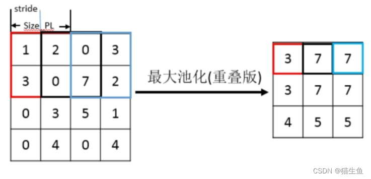
(图片来源在这里,感谢作者!)
全部代码
from torchvision.transforms import functional as F
import matplotlib.pyplot as plt
import torch.nn as nn
import cv2


# 将图片转换为模型可用的数据
def getImageData(imgFile):
    image = cv2.imread(imgFile, 0)
    image = F.to_tensor(image)  # shape为 [1, 768, 1024], [通道,高,宽]
    image = image.unsqueeze(0)  # shape为 [1, 1, 768, 1024], [数量,通道,高,宽]
    return image


# 将三个图片显示在plt上
def showTensorImg(image, title=""):
    plt.figure(title)  # 创建第一个图形
    plt.sca(plt.subplot(1, 3, 1))  # 分成1行2列,选择第1个位置
    plt.imshow(image[0].data, cmap=plt.cm.gray)
    plt.sca(plt.subplot(1, 3, 2))  # 分成1行2列,选择第2个位置
    plt.imshow(image[1].data, cmap=plt.cm.gray)
    plt.sca(plt.subplot(1, 3, 3))  # 分成1行2列,选择第2个位置
    plt.imshow(image[2].data, cmap=plt.cm.gray)


# 定义模型
class MyModel(nn.Module):
    def __init__(self):
        super(MyModel, self).__init__()
        self.conv0 = nn.Conv2d(in_channels=1, out_channels=3, kernel_size=(3, 3), stride=1, padding=1)
        self.relu0 = nn.ReLU(inplace=True)
        self.pool0 = nn.MaxPool2d(kernel_size=2, stride=1)

    # 把模型里的卷积层和激活层后的效果,显示出来看一看
    def forward(self, image):
        img = self.conv0(image)
        print("conv0:", img, img.shape, "\n")
        showTensorImg(img.squeeze(), "conv0")

        img = self.relu0(img)
        print("relu0:", img, img.shape, "\n")
        showTensorImg(img.squeeze(), "relu0")

        img = self.pool0(img)
        print("pool0:", img, img.shape, "\n")
        showTensorImg(img.squeeze(), "pool0")

        return img


if __name__ == "__main__":
    # 显示原图
    img = cv2.imread("Data/T.bmp", 0)
    plt.imshow(img)
    print(img.shape)

    net = MyModel()
    image = getImageData("Data/T.bmp")
    img = net(image)

    plt.show()


 1730
1730


 被折叠的 条评论
为什么被折叠?
被折叠的 条评论
为什么被折叠?
 到【灌水乐园】发言


