NNDL 作业9：分别使用numpy和pytorch实现BPTT

HBU_fangerfang

已于 2022-11-22 21:40:23 修改

阅读量383

点赞数 1

分类专栏：神经网络与深度学习文章标签： pytorch 深度学习人工智能

于 2022-11-22 21:40:11 首次发布

本文链接：https://blog.csdn.net/qq_33573422/article/details/127989428

版权

神经网络与深度学习专栏收录该内容

26 篇文章 2 订阅

订阅专栏

6-1P：推导RNN反向传播算法BPTT

6-2P：设计简单RNN模型，分别用Numpy、Pytorch实现反向传播算子，并代入数值测试

总结

6-1P：推导RNN反向传播算法BPTT

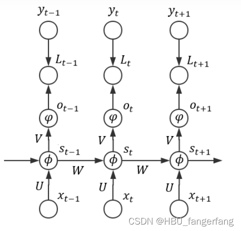
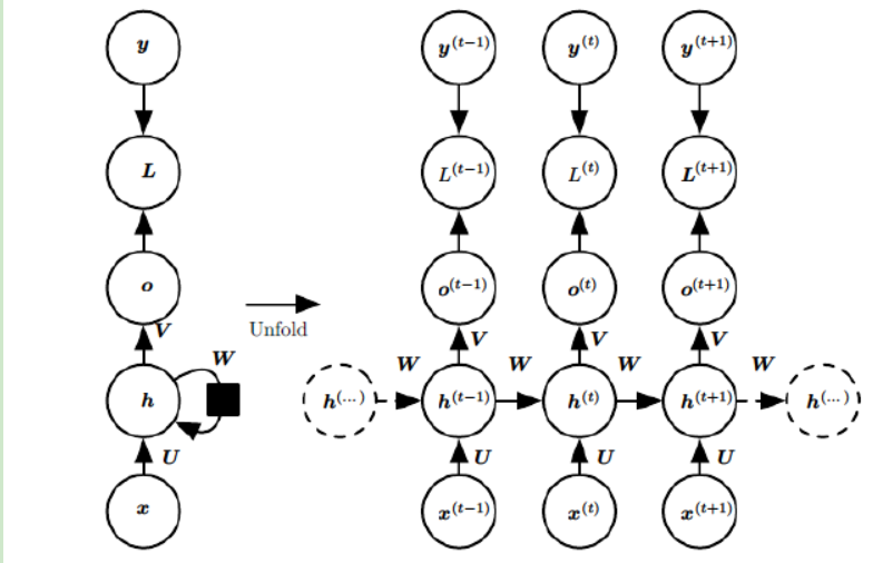
为了方便我们用以下朴素网络结构

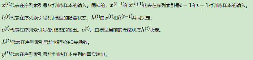
然后做出如下符号约定：

取ϕ作为隐藏层的激活函数
取φ作为输出层的变换函数
取 $L_t=L_t(o_t,y_t)$ 作为模型的损失函数，其中标签 $y_t$ 是一个one-hot 向量；由于 RNN 处理的通常是序列数据、所以在接受完序列中所有样本后再统一计算损失是合理的，此时模型的总损失可以表示为（假设输入序列长度为n）： $L=\sum^n_{t=1}L_t$

为了更清晰地表明各个配置，我们可以整理出如下图所示的结构：

易得 $o_t=\varphi (Vs_t)=\varphi (V\phi (Ux_i+Ws_{t-1}))$ ,其中 $s_0=0=(0,0,0....,0)^T$ 。

令： $o^*_t=Vs_t , s_t^*=Ux_t+Ws_{t-1}$

则有： $o_t=\varphi (o^*_t),s_t=\phi (s^*_t)$

从而:

$\frac{\partial L_t}{\partial o^*_t}=\frac{\partial L_t}{\partial o_t}\odot \frac{\partial o_t}{\partial o_t^*}=\frac{\partial L_t}{\partial o_t}\odot {\varphi}'(o_t^*)$

$\frac{\partial L_t}{\partial V}=\frac{\partial L_t}{\partial V_{s_t}} \times \frac{\partial V_{s_t}}{\partial V}=(\frac{\partial L_t}{\partial V_{s_t}}\odot {\varphi}'(o^*_t))\times s_t^T$

可见对矩阵V的分析过程即为普通的反向传播算法，相对而言比较平凡。由 $L=\sum^n_{t=1}L_t$ 可知，它的总梯度可以表示为： $\frac{\partial L}{\partial V}=\sum^n_{t=1}(\frac{\partial L_i}{\partial o_t}\odot {\varphi}'(o^*_t))\times s_t^T$

而事实上，RNN 的 BP 算法的主要难点在于它 State 之间的通信，亦即梯度除了按照空间结构传播（ot→st→xt）以外，还得沿着时间通道传播（st→st−1→…→s1），这导致我们比较难将相应 RNN 的 BP 算法写成一个统一的形式（回想之前的“前向传导算法”）。为此，我们可以采用“循环”的方法来计算各个梯度

由于是反向传播算法，所以t应从n开始降序循环至 1，在此期间（若需要初始化、则初始化为 0 向量或 0 矩阵）：

计算时间通道上的“局部梯度” ：

$\frac{\partial L_t}{\partial s_t^*}=\frac{\partial s_t}{\partial s_t^*}\odot (\frac{\partial s_t^*V^T}{\partial s_t}\times \frac{\partial L_t}{\partial Vs_t}) ={\phi}'(s^*_t)\odot [V^T\times (\frac{\partial L_t}{\partial o_t}\odot {\varphi}'(o^*_t))]$

$\frac{\partial L_t}{\partial s^*_{k-1}}=\frac{\partial s^*_k}{\partial s^*_{k-1}}\times \frac{\partial L_t}{\partial s^*_t}={\phi}'(s^*_{k-1})\odot (W^T\times \frac{\partial L_t}{\partial s^*_t}), (k=1,.......,t)$

利用时间通道上的“局部梯度”计算U和W的梯度：

以上即为 RNN 反向传播算法的所有推导，它比 NN 的 BP 算法要繁复不少。事实上，像这种需要把梯度沿时间通道传播的 BP 算法是有一个专门的名词来描述的——Back Propagation Through Time（常简称为 BPTT，可译为“时序反向传播算法”）

不妨举一个具体的栗子来加深理解，假设：

激活函数ϕ为 Sigmoid 函数
变换函数φ为 Softmax 函数
损失函数Lt为交叉熵损失函数

其中：

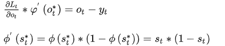
从而

且t从n开始降序循环至 1 的期间中，各个“局部梯度”为：

由此可算出如下相应梯度：

$\frac{\partial L_t}{\partial U}=\sum^t_{k=1}\frac{\partial L_t}{\partial s^*_k}\times x^T_k$

$\frac{\partial L_t}{\partial W}=\sum^t_{k=1}\frac{\partial L_t}{\partial s^*_k}\times s^T_{k-1}$

6-2P：设计简单RNN模型，分别用Numpy、Pytorch实现反向传播算子，并代入数值测试

Numpy实现：

class RNN:
    
    def __init__(self, word_dim, hidden_dim=100, bptt_truncate=4):
        self.word_dim = word_dim
        self.hidden_dim = hidden_dim
        self.bptt_truncate = bptt_truncate
        # Randomly initialize the network parameters, np.random.uniform(low,high,size=(m,n)) -> matrix: m * n
        self.U = np.random.uniform(-np.sqrt(1./word_dim), np.sqrt(1./word_dim), (hidden_dim, word_dim))
        self.V = np.random.uniform(-np.sqrt(1./hidden_dim), np.sqrt(1./hidden_dim), (word_dim, hidden_dim))
        self.W = np.random.uniform(-np.sqrt(1./hidden_dim), np.sqrt(1./hidden_dim), (hidden_dim, hidden_dim))

    def softmax(self,x):
        exp_x = np.exp(x)
        softmax_x = exp_x / np.sum(exp_x)
        return softmax_x

    def forward_propagation(self, x):
        # hidden states is h, prediction is y_hat
        T = len(x)
        h = np.zeros((T + 1, self.hidden_dim))
        h[-1] = np.zeros(self.hidden_dim)
        y_hat = np.zeros((T, self.word_dim))
        # For each time step...
        for t in np.arange(T):
            x_t = np.array(x[t]).reshape(-1,1)
            h[t] = (self.U.dot(x_t) + self.W.dot(h[t-1].reshape(-1,1))).reshape(self.hidden_dim)
            o_t = self.V.dot(h[t])
            y_hat[t] = self.softmax(o_t)
        return [y_hat, h]
  
    def predict(self, x):
        # Perform forward propagation and return index of the highest score
        y, h = self.forward_propagation(x)
        return np.argmax(y, axis=1)

    def calculate_total_loss(self, x, labels):
        total_L = 0
        # For each sentence...
        for i in np.arange(len(labels)):
            y_hat, h = self.forward_propagation(x[i])
            total_L += -1 * sum([np.log(y_pred.T.dot(y_true)) for y_pred,y_true in zip(y_hat,np.array(labels[i]))])
        return total_L
    
    def calculate_loss(self, x, labels):
        # Divide the total loss by the number of training examples
        N = np.sum((len(label_i) for label_i in labels))
        return self.calculate_total_loss(x,labels)/N

    def bptt(self, x, label):
        T = len(label)
        # Perform forward propagation
        y_hat, h = self.forward_propagation(x)
        # We accumulate the gradients in these variables
        dLdU = np.zeros(self.U.shape)
        dLdV = np.zeros(self.V.shape)
        dLdW = np.zeros(self.W.shape)
        # delta_y -> dLdy: y_hat_t - y_t
        delta_y = np.zeros(y_hat.shape)
        # For each output backwards...
        for t in np.arange(T)[::-1]:
            delta_y[t] = (y_hat[t].reshape(-1,1) - np.array(label[t]).reshape(-1,1)).ravel()
            dLdV += delta_y[t].reshape(-1,1).dot(h[t].T.reshape(1,-1))
            # Initial delta_t calculation when t is T
            delta_t = (1-(h[t]**2)) * self.V.T.dot(delta_y[t])
            # Backpropagation through time (for at most self.bptt_truncate steps)
            for bptt_step in np.arange(max(0, t-self.bptt_truncate), t+1)[::-1]:
                dLdW += delta_t * h[bptt_step-1] 
                dLdU += delta_t.reshape(-1,1) * np.array(x[bptt_step]).reshape(1,-1)          
                # Update delta_t for next step
                delta_t = (1-(h[t]**2)) * (self.V.T.dot(delta_y[bptt_step]) + self.W.T.dot(delta_t))
        return [dLdU, dLdV, dLdW]

    # Performs one step of SGD.
    def numpy_sdg_step(self, x, label, learning_rate):
        # Calculate the gradients
        dLdU, dLdV, dLdW = self.bptt(x, label)
        # Change parameters according to gradients and learning rate
        self.U -= learning_rate * dLdU
        self.V -= learning_rate * dLdV
        self.W -= learning_rate * dLdW
def train_with_sgd(model, X_train, y_train, learning_rate=0.005, nepoch=100, evaluate_loss_after=5):
    # We keep track of the losses so we can plot them later
    losses = []
    num_examples_seen = 0
    for epoch in range(nepoch):
        # Optionally evaluate the loss
        if (epoch % evaluate_loss_after == 0):
            loss = model.calculate_loss(X_train, y_train)
            losses.append((num_examples_seen, loss))
            time = datetime.now().strftime('%Y-%m-%d %H:%M:%S')
            print(f'{time} Loss after num_examples_seen {num_examples_seen} epoch {epoch}, current loss is {loss}')
            # Adjust the learning rate if loss increases
            if(len(losses)>1 and losses[-1][1]>losses[-2][1]):
                learning_rate = learning_rate * 0.5  
                print("Setting learning rate to %f" % learning_rate)
            sys.stdout.flush()
        # For each training example...
        for i in range(len(y_train)):
            # One SGD step
            model.numpy_sdg_step(X_train[i], y_train[i], learning_rate)
            num_examples_seen += 1
s1 = '你 好 李 焕 英'
s2 = '夏 洛 特 烦 恼'
vocab_size= len(s1.split(' ')) + len(s2.split(' '))
vocab = [[0] * vocab_size for _ in range(vocab_size)]
for i in range(vocab_size): vocab[i][i] = 1
x_sample = [vocab[:5]] + [vocab[5:]]
labels = [vocab[1:6]] + [vocab[6:]+[vocab[0]]]

rnn = RNN(10)
train_with_sgd(rnn,x_sample,labels)

得到以下结果：

Loss after num_examples_seen 0 epoch 0, current loss is 2.2592256714820835
Loss after num_examples_seen 10 epoch 5, current loss is 2.1503379839162173
Loss after num_examples_seen 20 epoch 10, current loss is 2.044293154297274
Loss after num_examples_seen 30 epoch 15, current loss is 1.940793510733868
Loss after num_examples_seen 40 epoch 20, current loss is 1.8396290861210651
Loss after num_examples_seen 50 epoch 25, current loss is 1.7406728454158427
Loss after num_examples_seen 60 epoch 30, current loss is 1.6438759771865512
Loss after num_examples_seen 70 epoch 35, current loss is 1.5492624544062168
Loss after num_examples_seen 80 epoch 40, current loss is 1.4569222603517766
Loss after num_examples_seen 90 epoch 45, current loss is 1.3670029019526193
Loss after num_examples_seen 100 epoch 50, current loss is 1.279699092774083
Loss after num_examples_seen 110 epoch 55, current loss is 1.1952407450521148
Loss after num_examples_seen 120 epoch 60, current loss is 1.1138796059742215
Loss after num_examples_seen 130 epoch 65, current loss is 1.0358749571871382
Loss after num_examples_seen 140 epoch 70, current loss is 0.9614787720174272
Loss after num_examples_seen 150 epoch 75, current loss is 0.8909206840507029
Loss after num_examples_seen 160 epoch 80, current loss is 0.8243932211561216
Loss after num_examples_seen 170 epoch 85, current loss is 0.7620381153394573
Loss after num_examples_seen 180 epoch 90, current loss is 0.7039350300238063
Loss after num_examples_seen 190 epoch 95, current loss is 0.650094418183265

Torch实现：

import torch
from torch import nn
import numpy as np
import matplotlib.pyplot as plt

plt.figure(figsize=(8, 5))

# how many time steps/data pts are in one batch of data
seq_length = 20

# generate evenly spaced data pts
time_steps = np.linspace(0, np.pi, seq_length + 1)
data = np.sin(time_steps)
data.resize((seq_length + 1, 1))  # size becomes (seq_length+1, 1), adds an input_size dimension

x = data[:-1]  # all but the last piece of data
y = data[1:]  # all but the first

# display the data
plt.plot(time_steps[1:], x, 'r.', label='input, x')  # x
plt.plot(time_steps[1:], y, 'b.', label='target, y')  # y

plt.legend(loc='best')
plt.show()


class RNN(nn.Module):
    def __init__(self, input_size, output_size, hidden_dim, n_layers):
        super(RNN, self).__init__()

        self.hidden_dim = hidden_dim

        # define an RNN with specified parameters
        # batch_first means that the first dim of the input and output will be the batch_size
        self.rnn = nn.RNN(input_size, hidden_dim, n_layers, batch_first=True)

        # last, fully-connected layer
        self.fc = nn.Linear(hidden_dim, output_size)

    def forward(self, x, hidden):
        # x (batch_size, seq_length, input_size)
        # hidden (n_layers, batch_size, hidden_dim)
        # r_out (batch_size, time_step, hidden_size)
        batch_size = x.size(0)

        # get RNN outputs
        r_out, hidden = self.rnn(x, hidden)
        # shape output to be (batch_size*seq_length, hidden_dim)
        r_out = r_out.view(-1, self.hidden_dim)

        # get final output
        output = self.fc(r_out)

        return output, hidden


# test that dimensions are as expected
test_rnn = RNN(input_size=1, output_size=1, hidden_dim=10, n_layers=2)

# generate evenly spaced, test data pts
time_steps = np.linspace(0, np.pi, seq_length)
data = np.sin(time_steps)
data.resize((seq_length, 1))

test_input = torch.Tensor(data).unsqueeze(0)  # give it a batch_size of 1 as first dimension
print('Input size: ', test_input.size())

# test out rnn sizes
test_out, test_h = test_rnn(test_input, None)
print('Output size: ', test_out.size())
print('Hidden state size: ', test_h.size())

# decide on hyperparameters
input_size = 1
output_size = 1
hidden_dim = 32
n_layers = 1

# instantiate an RNN
rnn = RNN(input_size, output_size, hidden_dim, n_layers)
print(rnn)

# MSE loss and Adam optimizer with a learning rate of 0.01
criterion = nn.MSELoss()
optimizer = torch.optim.Adam(rnn.parameters(), lr=0.01)


# train the RNN
def train(rnn, n_steps, print_every):
    # initialize the hidden state
    hidden = None

    for batch_i, step in enumerate(range(n_steps)):
        # defining the training data
        time_steps = np.linspace(step * np.pi, (step + 1) * np.pi, seq_length + 1)
        data = np.sin(time_steps)
        data.resize((seq_length + 1, 1))  # input_size=1

        x = data[:-1]
        y = data[1:]

        # convert data into Tensors
        x_tensor = torch.Tensor(x).unsqueeze(0)  # unsqueeze gives a 1, batch_size dimension
        y_tensor = torch.Tensor(y)

        # outputs from the rnn
        prediction, hidden = rnn(x_tensor, hidden)

        ## Representing Memory ##
        # make a new variable for hidden and detach the hidden state from its history
        # this way, we don't backpropagate through the entire history
        hidden = hidden.data

        # calculate the loss
        loss = criterion(prediction, y_tensor)
        # zero gradients
        optimizer.zero_grad()
        # perform backprop and update weights
        loss.backward()
        optimizer.step()

        # display loss and predictions
        if batch_i % print_every == 0:
            print('Loss: ', loss.item())
            plt.plot(time_steps[1:], x, 'r.')  # input
            plt.plot(time_steps[1:], prediction.data.numpy().flatten(), 'b.')  # predictions
            plt.show()

    return rnn


# train the rnn and monitor results
n_steps = 75
print_every = 15

trained_rnn = train(rnn, n_steps, print_every)

Input size:  torch.Size([1, 20, 1])
Output size:  torch.Size([20, 1])
Hidden state size:  torch.Size([2, 1, 10])
RNN(
  (rnn): RNN(1, 32, batch_first=True)
  (fc): Linear(in_features=32, out_features=1, bias=True)
)
Loss:  0.47356677055358887
Loss:  0.015861276537179947
Loss:  0.0011221482418477535
Loss:  0.0008511045016348362
Loss:  0.0004949825815856457

进程已结束，退出代码为 0