两种点云地面去除方法

最新推荐文章于 2023-04-26 08:54:55 发布

家门Jm

最新推荐文章于 2023-04-26 08:54:55 发布

阅读量1.3w

点赞数 32

分类专栏：点云相关

原文链接：https://adamshan.blog.csdn.net/article/details/84569000

版权

点云相关专栏收录该内容

3 篇文章 8 订阅

订阅专栏

1、基于角度分割的地面、非地面分割

1.1 PCL基本入门

1.1.1 在ROS项目中引入PCL库

1.2 编写节点进行Voxel Grid Filter

1.2.1 验证效果

1.3 点云地面过滤

1.3.1 点云剪裁和过滤——去除过高和过近的点

1.3.2 角度微分和地面/非地面判断——Ray Ground Filter

1.3.3 分割

2、基于地面平面拟合的激光雷达地面分割方法和ROS实现

2.1 地面平面拟合（Ground Plane Fitting）

本文参考自大佬博客：

1. https://adamshan.blog.csdn.net/article/details/82901295 《无人驾驶汽车系统入门（二十四）——激光雷达的地面-非地面分割和pcl_ros实践》

2. https://adamshan.blog.csdn.net/article/details/84569000 《无人驾驶汽车系统入门（二十七）——基于地面平面拟合的激光雷达地面分割方法和ROS实现》

1、基于角度分割的地面、非地面分割

在无人驾驶的雷达感知中，将雷达点云地面分割出来是一步基本的操作，这一步操作主要能够改善地面点对于地面以上的目标的点云聚类的影响。

本文首先带大家入门pcl_ros，首先我们使用pcl_ros编写一个简单的ros节点，对输入点云进行Voxel Grid Filter（体素滤波）。

1.1 PCL基本入门

PCL是一个开源的点云处理库，是在吸收了前人点云相关研究基础上建立起来的大型跨平台开源C++编程库，它实现了大量点云相关的通用算法和高效数据结构，包含点云获取、滤波、分割、配准、检索、特征提取、识别、追踪、曲面重建、可视化等大量开源代码。支持多种操作系统平台，可在Windows、Linux、Android、Mac OS X、部分嵌入式实时系统上运行。如果说OpenCV是2D信息获取与处理的结晶，那么PCL就在3D信息获取与处理上具有同等地位。ROS kinetic完整版中本身已经包含了pcl库，同时ROS自带的pcl_ros 包可以连接ROS和PCL库。我们从一个简单的Voxel Grid Filter的ROS节点实现来了解一下PCL在ROS中的基本用法，同时了解PCL中的一些基本数据结构：

1.1.1 在ROS项目中引入PCL库

在此我们假定读者已经自行安装好ROS kinetic 的完整版，首先在我们的catkin workspace中新建一个package，我们将它命名为pcl_test,可以通过如下指令生成workspace和package：

cd ~
mkdir -p pcl_ws/src
cd pcl_ws
catkin_make
source devel/setup.bash
cd src
catkin_create_pkg pcl_test roscpp sensor_msgs pcl_ros

这样，我们就新建了一个workspace，用于学习PCL，同时新建了一个名为pcl_test的package，这个ROS包依赖于roscpp，sensor_msgs, pcl_ros这几个包，我们修改pcl_test包下的CMakeList文件以及package.xml配置文件，如下：
package.xml 文件：

<?xml version="1.0"?>
<package>
  <name>pcl_test</name>
  <version>0.0.1</version>
  <description>The pcl_test package</description>


  <maintainer email="shenzb12@lzu.edu.cn">adam</maintainer>

  <license>MIT</license>


  <buildtool_depend>catkin</buildtool_depend>
  <build_depend>roscpp</build_depend>
  <build_depend>sensor_msgs</build_depend>
  <build_depend>pcl_ros</build_depend>

  <run_depend>roscpp</run_depend>
  <run_depend>sensor_msgs</run_depend>
  <run_depend>pcl_ros</run_depend>
</package>

CMakeList.txt 文件：

cmake_minimum_required(VERSION 2.8.3)
project(pcl_test)

add_compile_options(-std=c++11)


find_package(catkin REQUIRED COMPONENTS
pcl_ros
roscpp
sensor_msgs
)


catkin_package(
  INCLUDE_DIRS include
  CATKIN_DEPENDS roscpp sensor_msgs pcl_ros
)

include_directories(
 include
 ${catkin_INCLUDE_DIRS}
)
link_directories(${PCL_LIBRARY_DIRS})


add_executable(${PROJECT_NAME}_node src/pcl_test_node.cpp src/pcl_test_core.cpp)


target_link_libraries(${PROJECT_NAME}_node
  ${catkin_LIBRARIES}
  ${PCL_LIBRARIES}
)

package.xml的内容很简单，实际上就是这个包的描述文件，build_depend 和 run_depend 两个描述符分别指定了程序包编译和运行的依赖项，通常是所用到的库文件的名称。在这里我们指定了三个编译和运行时依赖项，分别是roscpp（编写C++ ROS节点），sensor_msgs（定义了激光雷达的msg），pcl_ros（连接ROS和pcl库）。

同样的，在CMakeList中，我们通过find_package查找这三个包的路径，然后将三个包添加到 CATKIN_DEPENDS, 在使用pcl库前，需要将PCL库的路径链接，通过link_directories(${PCL_LIBRARY_DIRS})来完成，并在最后的target_link_libraries中添加${PCL_LIBRARIES}。

1.2 编写节点进行Voxel Grid Filter

接着我们在pcl_test/src目录下新建pcl_test_node.cpp文件：

#include "pcl_test_core.h"     // 自己写的头文件

int main(int argc, char **argv)
{
    ros::init(argc, argv, "pcl_test");

    ros::NodeHandle nh;

    PclTestCore core(nh);
    
    return 0;
}

此文件仅包含main函数，是节点的入口，编写头文件include/pcl_test_core.h:

#pragma once

#include <ros/ros.h>

#include <pcl_conversions/pcl_conversions.h>
#include <pcl/point_types.h>
#include <pcl/conversions.h>
#include <pcl_ros/transforms.h>

#include <pcl/filters/voxel_grid.h>

#include <sensor_msgs/PointCloud2.h>

class PclTestCore
{

private:
    ros::Subscriber sub_point_cloud_;

    ros::Publisher pub_filtered_points_;

    void point_cb(const sensor_msgs::PointCloud2ConstPtr& in_cloud);

public:
    PclTestCore(ros::NodeHandle &nh);
    ~PclTestCore();
    void Spin();
};

以及pcl_test_core.cpp：

#include "pcl_test_core.h"

PclTestCore::PclTestCore(ros::NodeHandle &nh)
{
    sub_point_cloud_ = nh.subscribe("/velodyne_points",10, &PclTestCore::point_cb, this);

    pub_filtered_points_ = nh.advertise<sensor_msgs::PointCloud2>("/filtered_points", 10);

    ros::spin();
}

PclTestCore::~PclTestCore(){}

void PclTestCore::Spin()
{
    
}

void PclTestCore::point_cb(const sensor_msgs::PointCloud2ConstPtr& in_cloud_ptr)
{
    pcl::PointCloud<pcl::PointXYZI>::Ptr current_pc_ptr(new pcl::PointCloud<pcl::PointXYZI>);
    pcl::PointCloud<pcl::PointXYZI>::Ptr filtered_pc_ptr(new pcl::PointCloud<pcl::PointXYZI>);

    pcl::fromROSMsg(*in_cloud_ptr, *current_pc_ptr);

    pcl::VoxelGrid<pcl::PointXYZI> vg;

    vg.setInputCloud(current_pc_ptr);
    vg.setLeafSize(0.2f, 0.2f, 0.2f);
    vg.filter(*filtered_pc_ptr);

    sensor_msgs::PointCloud2 pub_pc;
    pcl::toROSMsg(*filtered_pc_ptr, pub_pc);

    pub_pc.header = in_cloud_ptr->header;

    pub_filtered_points_.publish(pub_pc);
}

这个节点的功能是订阅来自/velodyne_points话题的点云数据，使用PCL内置的Voxel Grid Filter对原始点云进行降采样，将降采样的结构发布到/filtered_points话题上。我们重点看回调函数PclTestCore::point_cb。在该回调函数中，我们首先定义了两个点云指针，在PCL库中，pcl::PointCloud<T>是最基本的一种数据结构，它表示一块点云数据（点的集合），我们可以指定点的数据结构，在上述实例中，采用了pcl::PointXYZI这种类型的点。pcl::PointXYZI结构体使用(x, y, z, intensity)这四个数值来描述一个三维度空间点。

intensity，即反射强度，是指激光雷达的激光发射器发射激光后收到的反射的强度，通常所说的16线，32线激光雷达，其内部实际是并列纵排的多个激光发射器，通过电机自旋，产生360环视的点云数据，不同颜色的物体对激光的反射强度也是不同的，通常来说，白色物体的反射强度（intensity）最强，对应的，黑色的反射强度最弱。

通常使用sensor_msgs/PointCloud2.h 做为点云数据的消息格式，可使用pcl::fromROSMsg和pcl::toROSMsg将sensor_msgs::PointCloud2与pcl::PointCloud<T>进行转换，这里的T就是pcl::PointXYZI。

为了使用Voxel Grid Filter对原始点云进行降采样，只需定义pcl::VoxelGrid并且指定输入点云和leaf size，在本例中，我们使用leaf size为 0.2。Voxel Grid Filter将输入点云使用0.2m*0.2m*0.2m的立方体进行分割，使用小立方体的形心（centroid）来表示这个立方体的所有点，保留这些点作为降采样的输出。

1.2.1 验证效果

我们写一个launch文件pcl_test.launch来启动这个节点：

<launch>
    <node pkg="pcl_test" type="pcl_test_node" name="pcl_test_node" output="screen"/>
</launch>

回到workspace 目录，使用catkin_make 编译：

catkin_make

启动这个节点：

roslaunch pcl_test pcl_test.launch

新建终端，并运行我们的测试bag（测试bag下载链接：https://pan.baidu.com/s/1HOhs9StXUmZ_5sCALgKG3w）

rosbag play --clock test.bag

打开第三个终端，启动Rviz：

rosrun rviz rviz

配置Rviz的Frame为velodyne，并且加载原始点云和过滤以后的点云的display：

在这里插入图片描述

原始点云：

在这里插入图片描述

降采样之后的点云（即我们的节点的输出）：

在这里插入图片描述

1.3 点云地面过滤

过滤地面是激光雷达感知中一步基础的预处理操作，因为我们环境感知通常只对路面上的障碍物感兴趣，且地面的点对于障碍物聚类容易产生影响，所以在做Lidar Obstacle Detection之前通常将地面点和非地面点进行分离。在此文中我们介绍一种被称为Ray Ground Filter的路面过滤方法，并且在ROS中实践。

1.3.1 点云剪裁和过滤——去除过高和过近的点

要分割地面和非地面，那么过高的区域首先就可以忽略不计，我们先对点云进行高度的裁剪。我们实验用的bag在录制的时候lidar的高度约为1.78米，我们剪裁掉1.28米以上的部分，代码如下：

void PclTestCore::clip_above(double clip_height, const pcl::PointCloud<pcl::PointXYZI>::Ptr in,
                             const pcl::PointCloud<pcl::PointXYZI>::Ptr out)
{
    pcl::ExtractIndices<pcl::PointXYZI> cliper;

    cliper.setInputCloud(in);
    pcl::PointIndices indices;
#pragma omp for    // 开启线程同步
    for (size_t i = 0; i < in->points.size(); i++)
    {
        if (in->points[i].z > clip_height)   // 挑选出高于阈值的
        {
            indices.indices.push_back(i);
        }
    }
    cliper.setIndices(boost::make_shared<pcl::PointIndices>(indices));
    cliper.setNegative(true); //ture to remove the indices 去除高于阈值的
    cliper.filter(*out);
}

为了消除车身自身的雷达反射的影响，我们对近距离的点云进行过滤，仍然使用pcl::ExtractIndices进行剪裁：

void PclTestCore::remove_close_pt(double min_distance, const pcl::PointCloud<pcl::PointXYZI>::Ptr in,
                                  const pcl::PointCloud<pcl::PointXYZI>::Ptr out)
{
    pcl::ExtractIndices<pcl::PointXYZI> cliper;

    cliper.setInputCloud(in);
    pcl::PointIndices indices;
#pragma omp for
    for (size_t i = 0; i < in->points.size(); i++)
    {
        double distance = sqrt(in->points[i].x*in->points[i].x + in->points[i].y*in->points[i].y);

        if (distance < min_distance)
        {
            indices.indices.push_back(i);
        }
    }
    cliper.setIndices(boost::make_shared<pcl::PointIndices>(indices));
    cliper.setNegative(true); //ture to remove the indices
    cliper.filter(*out);
}

其中，#pragma omp for语法OpenMP的并行化语法，即希望通过OpenMP并行化执行这条语句后的for循环，从而起到加速的效果。

1.3.2 角度微分和地面/非地面判断——Ray Ground Filter

Ray Ground Filter算法的核心是以射线（Ray）的形式来组织点云。我们现在将点云的 (x, y, z)三维空间降到（x,y）平面来看，计算每一个点到车辆x正方向的平面夹角 θ, 我们对360度进行微分，分成若干等份，每一份的角度为0.18度，这个微分的等份近似的可以看作一条射线，如下图所示,图中是一个激光雷达的纵截面的示意图，雷达由下至上分布多个激光器，发出如图所示的放射状激光束，这些激光束在平地上即表现为，图中的水平线即为一条射线：

0.18度是VLP32C雷达的水平光束发散间隔。

为了方便地对点进行半径和夹角的表示，我们使用如下数据结构代替pcl::PointCloudXYZI：

struct PointXYZIRTColor
{
    pcl::PointXYZI point;

    float radius; //cylindric coords on XY Plane
    float theta;  //angle deg on XY plane

    size_t radial_div;     //index of the radial divsion to which this point belongs to
    size_t concentric_div; //index of the concentric division to which this points belongs to

    size_t original_index; //index of this point in the source pointcloud
};

typedef std::vector<PointXYZIRTColor> PointCloudXYZIRTColor;

其中，radius表示点到lidar的水平距离(半径)，即：

theta是点相对于车头正方向(即x方向)的夹角，计算公式为：

我们用radial_div和concentric_div分别描述角度微分和距离微分。对点云进行水平角度微分之后，可得到：360/0.18 = 2000条射线，将这些射线中的点按照距离的远近进行排序，如下所示：

    //将同一根射线上的点按照半径（距离）排序
#pragma omp for
    for (size_t i = 0; i < radial_dividers_num_; i++)
    {
        std::sort(out_radial_ordered_clouds[i].begin(), out_radial_ordered_clouds[i].end(),[](const PointXYZIRTColor &a, const PointXYZIRTColor &b) { return a.radius < b.radius; });
    }

通过判断射线中前后两点的坡度是否大于我们事先设定的坡度阈值，从而判断点是否为地面点。代码如下：

void PclTestCore::classify_pc(std::vector<PointCloudXYZIRTColor> &in_radial_ordered_clouds,
                              pcl::PointIndices &out_ground_indices,
                              pcl::PointIndices &out_no_ground_indices)
{
    out_ground_indices.indices.clear();         // 地面点
    out_no_ground_indices.indices.clear();      // 非地面点

#pragma omp for
    // sweep through each radial division 遍历每一根射线
    for( size_t i=0; i < in_radial_ordered_clouds.size(); i ++ )
    {
        float prev_radius = 0.f;
        float prev_height = -SENSOR_HEIGHT;
        bool  prev_ground = false;
        bool  current_ground = false;

        // 遍历每一个射线上的所有点
        for( size_t j=0; j<in_radial_ordered_clouds[i].size(); j ++ )
        {
            float points_distance  = in_radial_ordered_clouds[i][j].radius - prev_radius;   // 与前一个点的距离
            float height_threshold = tan(DEG2RAD(local_max_slope_)) * points_distance;
            float current_height = in_radial_ordered_clouds[i][j].point.z;      // 当前点的实际z值
            float general_height_threshold = tan(DEG2RAD(general_max_slope_)) * in_radial_ordered_clouds[i][j].radius;

            // for points which are very close causing the height threshold to be tiny, set a minimum value
            // 对于非常接近导致高度阈值很小的点，请设置一个最小值
            if ( points_distance > concentric_divider_distance_ && height_threshold < min_height_threshold_ )
            {
                height_threshold = min_height_threshold_;
            }

            // check current point height against the LOCAL threshold (previous point)  对照局部阈值检查当前点高度（上一点）
            if ( current_height <= (prev_height+height_threshold) && current_height >= (prev_height-height_threshold) )
            {
                // check again using general geometry (radius from origin) if previous points wasn't ground
                if ( !prev_ground )     // 前一点不是地面点，需要进一步判断当前点
                {
                    if (current_height <= (-SENSOR_HEIGHT+general_height_threshold) && current_height >= (-SENSOR_HEIGHT-general_height_threshold))
                    {
                        current_ground = true;
                    }
                    else
                    {
                        current_ground = false;
                    }
                }
                else    // 上一点是地面点，当前点在上一点阈值高度范围内，所以这一点一定是地面点
                {
                    current_ground = true;
                }
            }
            else
            {
                // check if previous point is too far from previous one, if so classify again
                // 检查当前点是否离上一个点太远，如果是，重新分类
                if ( points_distance > reclass_distance_threshold_ &&
                     (current_height <= (-SENSOR_HEIGHT+height_threshold) && current_height >= (-SENSOR_HEIGHT-height_threshold)))
                {
                    current_ground = true;
                }
                else
                {
                    current_ground = false;
                }
            }

            // 最终判断当前点是否为地面点
            if ( current_ground )
            {
                out_ground_indices.indices.push_back(in_radial_ordered_clouds[i][j].original_index);
                prev_ground = true;
            }
            else
            {
                out_no_ground_indices.indices.push_back(in_radial_ordered_clouds[i][j].original_index);
                prev_ground = false;
            }

            prev_radius = in_radial_ordered_clouds[i][j].radius;
            prev_height = in_radial_ordered_clouds[i][j].point.z;
        }
    }

}

这里有两个重要参数，一个是local_max_slope_，是我们设定的同条射线上邻近两点的坡度阈值，一个是general_max_slope_，表示整个地面的坡度阈值，这两个坡度阈值的单位为度（degree），我们通过这两个坡度阈值以及当前点的半径（到lidar的水平距离）求得高度阈值，通过判断当前点的高度（即点的z值）是否在地面加减高度阈值范围内来判断当前点是为地面。

在地面判断条件中，current_height <= (-SENSOR_HEIGHT + general_height_threshold) && current_height >= (-SENSOR_HEIGHT - general_height_threshold) 中SENSOR_HEIGHT表示lidar挂载的高度，-SNESOR_HEIGHT即表示水平地面。

1.3.3 分割

我们使用上文中的bag来验证地面分割节点的工作效果。运行bag并且运行我们的节点，打开Rviz，加载两个点云display，效果如下所示：

在这里插入图片描述

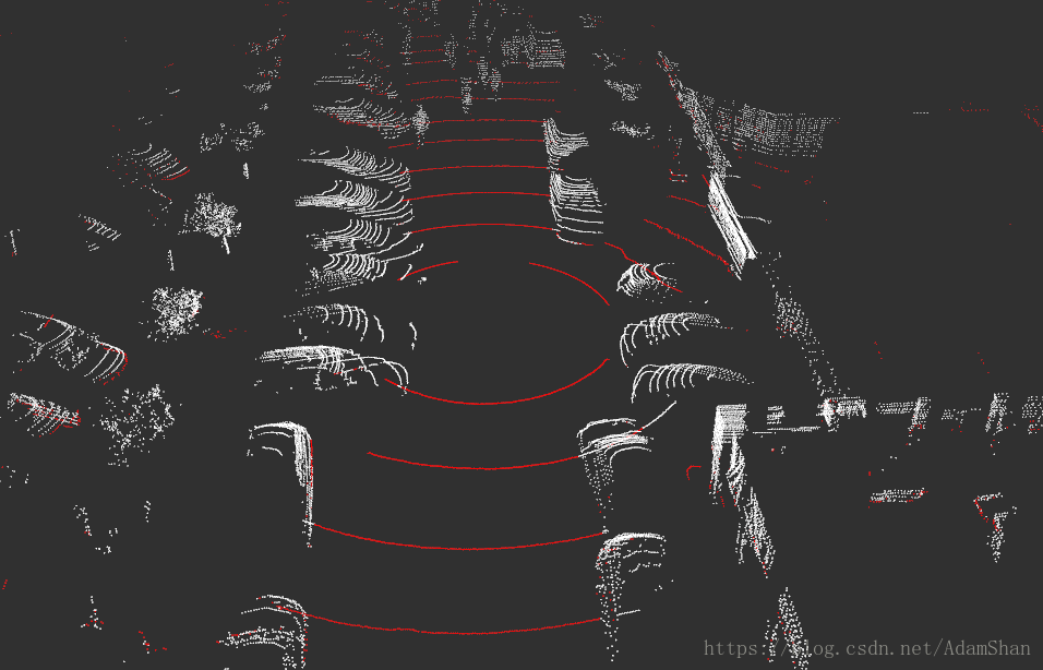
其中，红色的点为我们分割出来的地面，来自于 /filtered_points_ground 话题，白色的点为非地面，来自于 /filtered_points_no_ground 话题。分割出非地面点云之后，我们就可以让Lidar Detection的代码工作在这个点云上了，从而排除了地面对于Lidar聚类以及Detection的影响。

2、基于地面平面拟合的激光雷达地面分割方法和ROS实现

上面是一种基于射线的地面过滤方法，此方法能够很好的完成地面分割，但是存在几点不足：

第一，存在少量噪点，不能彻底过滤出地面；
第二，非地面的点容易被错误分类，造成非地面点缺失；
第三，对于目标接近激光雷达盲区的情况，会出现误分割，即将非地面点云分割为地面。

通过本文我们一起学习一种新的地面分割方法，出自论文：Fast segmentation of 3D point clouds: A paradigm on LiDAR data for autonomous vehicle applications，在可靠性、分割精度方面均优于基于射线的地面分割方法。我们将其称之为地面平面拟合方法。

2.1 地面平面拟合（Ground Plane Fitting）

我们采用平面模型（Plane Model）来拟合当前的地面，通常来说，由于现实的地面并不是一个“完美的”平面，而且当距离较大时激光雷达会存在一定的测量噪声，单一的平面模型并不足以描述我们现实的地面。

要很好的完成地面分割，就必须要处理存在一定坡度变化的地面的情况（不能将这种坡度的变化视为非地面，不能因为坡度的存在而引入噪声），一种简单的处理方法就是沿着x方向（车头的方向）将空间分割成若干个子平面，然后对每个子平面使用地面平面拟合算法（GPF）从而得到能够处理陡坡的地面分割方法。

那么如何进行平面拟合呢？其伪代码如下：

在这里插入图片描述

我们来详细的了解这一流程：对于给定的点云 P ,分割的最终结果为两个点云集合 $P_{g}$ ：地面点云和 $P_{ng}$ ：非地面点云。该算法有四个重要的参数，分别是：

$N_{iter}$ ：进行奇异值分解（singular value decomposition，SVD）的次数，也即进行优化拟合的次数；
$N_{LPR}$ ：用于选取LPR的最低高度点的数量；
$Th_{seed}$ ：用于选取种子点的阈值，当点云内的点的高度小于LPR的高度加上此阈值时，我们将该点加入种子点集；
$Th_{dist}$ ：平面距离阈值，我们会计算点云中每一个点到我们拟合的平面的正交投影的距离，而这个平面距离阈值，就是用来判定点是否属于地面。

2.2 种子点集选取

我们首先选取一个种子点集(seed point set)，这些种子点来源于点云中高度（即z值）较小的点，种子点集被用于建立描述地面的初始平面模型，那么如何选取这个种子点集呢？

我们引入最低点代表（Lowest Point Representative, LPR）的概念。LPR就是 $N_{LPR}$ 个最低高度点的平均值，LPR 保证了平面拟合阶段不受测量噪声的影响。这个LPR被当作是整个点云 P 的最低点，点云P中高度在阈值 $Th_{seed}$ 内的点被当作是种子点，由这些种子点构成一个种子点集合。

种子点集的选取代码如下：

void PlaneGroundFilter::extract_initial_seeds_(const pcl::PointCloud<VPoint> &p_sorted)
{
    // LPR is the mean of low point representative.
    double sum = 0;     //
    int cnt = 0;        // 点云计数

    // Calculate the mean height value. 因为已经排过序了，所以直接选取前最小的num_lpr个点即可
    for( int i=0; i<p_sorted.points.size() && cnt<num_lpr_; i ++ )
    {
        sum += p_sorted.points[i].z;
        cnt ++;
    }

    double lpr_height = cnt != 0 ? sum / cnt : 0;   // in case divide by 0
    g_seeds_pc->clear();

    // iterate pointcloud, filter those height is less than lpr.height + th_seeds_.  得到初始地面种子点
    for( int i=0; i<p_sorted.points.size(); i ++ )
    {
        if ( p_sorted.points[i].z < lpr_height + th_seeds_ )
        {
            g_seeds_pc->points.push_back(p_sorted.points[i]);
        }
    }

    // return seeds points
}

输入是一个点云，这个点云内的点已经沿着z方向（即高度）做了排序，取 num_lpr_ 个最小点，求得高度平均值 lpr_height（即LPR），选取高度小于 lpr_height + th_seeds_ 的点作为种子点。

2.3 平面模型

接下来我们需要确定一个平面，点云中的点到这个平面的正交投影距离小于阈值 $Th_{dist}$ 则认为该点属于地面，否则属于非地面，我们采用一个简单的线性模型用于平面模型估计，如下：
ax+by+cz+d = 0

也即：

其中， $\hat{s}$ 是所有点的均值。这个协方差矩阵 C 描述了种子点集的散布情况，其三个奇异向量可以通过奇异值分解（Singular Value Decomposition,SVD）求得，这三个奇异向量描述了点集在三个主要方向的散布情况。由于是平面模型，垂直于平面的法向量n表示具有最小方差的方向，可以通过计算具有最小奇异值的奇异向量来求得。

那么在求得了 n 以后， d 可以通过代入种子点集的平均值 $\hat{s}$ (它代表属于地面的点) 直接求得。整个平面模型计算代码如下：

// 根据ax+by+cz+d = 0，拟合平面，最重要的是确定点与平面的投影距离阈值Th_dist，并以此判断点是否在平面上
void PlaneGroundFilter::estimate_plane_(void)
{
    // Create covariance matrix in single pass.
    // TODO: compare the efficiency.
    Eigen::Matrix3f cov;
    Eigen::Vector4f pc_mean;

    // 计算均值和协方差矩阵
    pcl::computeMeanAndCovarianceMatrix(*g_ground_pc, cov, pc_mean);

    // Singular Value Decomposition: SVD  奇异值分解
    JacobiSVD<MatrixXf> svd(cov, Eigen::DecompositionOptions::ComputeFullU);

    // use the least singular vector as normal.     取前三维作为主要方向：U矩阵m*m => m*r r=3  m是g_ground_pc点云的点数
    normal_ = (svd.matrixU().col(2));

    // mean ground seeds value.
    Eigen::Vector3f seeds_mean = pc_mean.head<3>();     // 要XYZIR前三维，XYZ


    // according to normal.T * [x, y, z] = -d
    d_ = -(normal_.transpose() * seeds_mean)(0, 0);
    // set distance threshold to 'th_dist - d'
    // 点云中的点到这个平面的正交投影距离小于阈值 Th_dist, 则认为该点属于地面，否则属于非地面
    th_dist_d_ = th_dist_ - d_;

    // return the equation parameters.
}

2.4 优化平面主循环

在确定如何选取种子点集以及如何估计平面模型以后，我们来看一下整个算法的主循环，以下是主循环的代码：

    // 4. Extract init ground seeds.  提取初始地面点
    extract_initial_seeds_(laserCloudIn);
    g_ground_pc = g_seeds_pc;


    // 5. Ground plane fitter mainloop
    for(int i=0; i<num_iter_; i ++)
    {
        estimate_plane_();          // 用上面 估计的g_ground_pc点云 来拟合地平面
        g_ground_pc->clear();       // 准备重新来得到地面点云，用以进行下一次平面拟合
        //g_not_ground_pc->clear();

        // pointcloud to matrix  点云数据转换为矩阵存储 n*3维度表示
        MatrixXf points(laserCloudIn_org.points.size(), 3);
        int j = 0;
        for(auto p : laserCloudIn_org.points)
        {
            points.row(j ++) << p.x, p.y, p.z;
        }

        // ground plane model  所有点与地平面法线的点乘，得到与地平面的距离
        VectorXf result = points * normal_;
        // threshold filter
        for (int r = 0; r < result.rows(); ++r)
        {
            if( result[r] < th_dist_d_ )    // 距离小于阈值的，就划分为地平面
            {
                g_all_pc->points[r].label = 1u;     // mean ground 表示地面，在所有点云中进行标签标识，加以区分
                g_ground_pc->points.push_back(laserCloudIn_org[r]);     // 单独存放地面点云
            }
            else
            {
                g_all_pc->points[r].label = 0u;     // mean not ground and non clustered
                g_not_ground_pc->points.push_back(laserCloudIn_org[r]); // 单独存放非地面点云
            }
        }
    }

得到这个初始的平面模型以后，我们会计算点云中每一个点到该平面的正交投影的距离，即 points * normal_，并且将这个距离与设定的阈值 $Th_{dist}$ （即th_dist_d_）比较，当高度差小于此阈值，我们认为该点属于地面，当高度差大于此阈值，则为非地面点。经过分类以后的所有地面点被当作下一次迭代的种子点集，迭代优化。

2.5 点云过滤

下面我们编写一个简单的ROS节点实现这一地面分割算法。我们仍然采用第24篇博客（激光雷达的地面-非地面分割和pcl_ros实践）中的bag进行实验，这个bag来自Velodyne的VLP32C，在此算法的基础上我们要进一步滤除雷达过近处和过高处的点，因为雷达安装位置的原因，近处的车身反射会对Detection造成影响，需要滤除; 过高的目标，如大树、高楼，对于无人车的雷达感知意义也不大，我们对过近过高的点进行切除，代码如下：

// 去除过近或者过远的点
void PlaneGroundFilter::remove_close_far_pt(const pcl::PointCloud<VPoint>::Ptr in,
                                            const pcl::PointCloud<VPoint>::Ptr out)
{
    pcl::ExtractIndices<VPoint> cliper;
    pcl::PointIndices indices;

#pragma omp for
    for( size_t i=0; i < in->points.size(); i ++ )
    {
        double distance = sqrt(in->points[i].x*in->points[i].x + in->points[i].y*in->points[i].y);

        if( (distance < min_distance_) || (distance > max_distance_) )
        {
            indices.indices.push_back(i);
        }
    }
    cliper.setIndices(boost::make_shared<pcl::PointIndices>(indices));
    cliper.setNegative(true);       // true to remove the indices
    cliper.filter(*out);
}

2.6 整体流程

主要流程都在PlaneGroundFilter::point_cb()函数中：

1. 数据预处理，将输入的Msg消息转换成pcl::pointcloud，并将点云全部存入g_all_pc中：

// 主要处理函数
void PlaneGroundFilter::point_cb(const sensor_msgs::PointCloud2ConstPtr &in_cloud_ptr)
{
    // 1. Msg to pointcloud  数据类型转换
    pcl::PointCloud<VPoint> laserCloudIn;
    pcl::fromROSMsg(*in_cloud_ptr, laserCloudIn);

    pcl::PointCloud<VPoint> laserCloudIn_org;
    pcl::fromROSMsg(*in_cloud_ptr, laserCloudIn_org);
    // For mark ground points and hold all points.
    SLRPointXYZIRL point;

    // 将输入的所有点存放到g_all_pc中
    for(size_t i=0; i < laserCloudIn.points.size(); i ++)
    {
        point.x = laserCloudIn.points[i].x;
        point.y = laserCloudIn.points[i].y;
        point.z = laserCloudIn.points[i].z;
        point.intensity = laserCloudIn.points[i].intensity;
        point.ring = laserCloudIn.points[i].ring;
        point.label = 0u;       // 0 means uncluster.
        g_all_pc->points.push_back(point);
    }

2. 对点云按照z轴数值大小对输入点云进行排序：

    // 2. Sort on Z-axis value.  按照z轴数值大小对输入点云进行排序
    sort(laserCloudIn.points.begin(), laserCloudIn.end(), point_cmp);

3. 对Z轴数据过小的点直接去除：

    // 3. Error point removal  清除一部分错误点
    // As there are some error mirror reflection under the ground,
    // here regardless point under 2* sensor_height
    // Sort point according to height, here uses z-axis in default
    pcl::PointCloud<VPoint>::iterator it = laserCloudIn.points.begin();
    for( int i=0; i < laserCloudIn.points.size(); i ++ )
    {
        if( laserCloudIn.points[i].z < -1.5*sensor_height_ )
        {
            it ++;
        }
        else
        {
            break;
        }
    }
    laserCloudIn.points.erase(laserCloudIn.points.begin(), it);

4. 提取初始地面种子点

    // 4. Extract init ground seeds.  提取初始地面点
    extract_initial_seeds_(laserCloudIn);
    g_ground_pc = g_seeds_pc;

5. 地面去除主循环

    // 5. Ground plane fitter mainloop
    for(int i=0; i<num_iter_; i ++)
    {
        estimate_plane_();          // 用上面 估计的g_ground_pc点云 来拟合地平面
        g_ground_pc->clear();       // 准备重新来得到地面点云，用以进行下一次平面拟合
        //g_not_ground_pc->clear();

        // pointcloud to matrix  点云数据转换为矩阵存储 n*3维度表示
        MatrixXf points(laserCloudIn_org.points.size(), 3);
        int j = 0;
        for(auto p : laserCloudIn_org.points)
        {
            points.row(j ++) << p.x, p.y, p.z;
        }

        // ground plane model  所有点与地平面法线的点乘，得到与地平面的距离
        VectorXf result = points * normal_;
        // threshold filter
        for (int r = 0; r < result.rows(); ++r)
        {
            if( result[r] < th_dist_d_ )    // 距离小于阈值的，就划分为地平面
            {
                g_all_pc->points[r].label = 1u;     // mean ground 表示地面，在所有点云中进行标签标识，加以区分
                g_ground_pc->points.push_back(laserCloudIn_org[r]);     // 单独存放地面点云
            }
            else
            {
                g_all_pc->points[r].label = 0u;     // mean not ground and non clustered
                g_not_ground_pc->points.push_back(laserCloudIn_org[r]); // 单独存放非地面点云
            }
        }
    }

6. 对去除地面点后的点云进行后处理：

    // 6. 对去除地面的点云进行后处理
    pcl::PointCloud<VPoint>::Ptr final_no_ground(new pcl::PointCloud<VPoint>);
    post_process(g_not_ground_pc, final_no_ground);

    // ROS_INFO_STREAM("origin: "<<g_not_ground_pc->points.size()<<" post_process: "<<final_no_ground->points.size());

    // publish ground points        发布地面点云
    sensor_msgs::PointCloud2 ground_msg;
    pcl::toROSMsg(*g_ground_pc, ground_msg);
    ground_msg.header.stamp = in_cloud_ptr->header.stamp;           // 时间戳
    ground_msg.header.frame_id = in_cloud_ptr->header.frame_id;     // 帧Id
    pub_ground_.publish(ground_msg);

    // publish not ground points    发布非地面点云
    sensor_msgs::PointCloud2 groundless_msg;
    pcl::toROSMsg(*final_no_ground, groundless_msg);
    //pcl::toROSMsg(*g_not_ground_pc, groundless_msg);
    groundless_msg.header.stamp = in_cloud_ptr->header.stamp;           // 时间戳
    groundless_msg.header.frame_id = in_cloud_ptr->header.frame_id;     // 帧Id
    pub_no_ground_.publish(groundless_msg);

    // publish all points           发布所有点云
    sensor_msgs::PointCloud2 all_points_msg;
    pcl::toROSMsg(*g_all_pc, all_points_msg);
    all_points_msg.header.stamp = in_cloud_ptr->header.stamp;
    all_points_msg.header.frame_id = in_cloud_ptr->header.frame_id;
    pub_all_points_.publish(all_points_msg);
    g_all_pc->clear();
}

家门Jm

关注

32
点赞
踩
245

收藏

觉得还不错? 一键收藏
3
评论
两种点云地面去除方法

本文参考自大佬博客：1.https://adamshan.blog.csdn.net/article/details/82901295《无人驾驶汽车系统入门（二十四）——激光雷达的地面-非地面分割和pcl_ros实践》2.https://adamshan.blog.csdn.net/article/details/84569000《无人驾驶汽车系统入门（二十七）——基于地面平面拟合的激光雷达地面分割方法和ROS实现》1、基于角度分割的地面、非地面分割...
复制链接

扫一扫