Python图像纹理分割

1️⃣作业要求

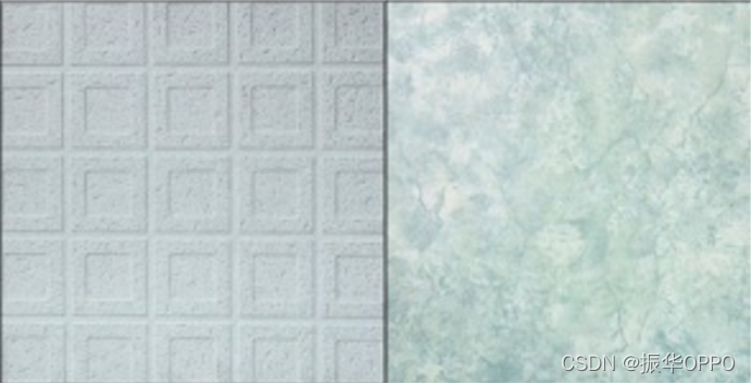
将下图左右两种不同类型的纹理区域分开，方法输出结果是一幅与该图像等大小的二值图像，左边为0，右边为1，或者相反，灰色边框线在设计的方法中不作考虑，自行去除。

2️⃣实现源码

import matplotlib.image as mpimg
import matplotlib.pyplot as plt
import numpy as np
from cv2 import cv2
from sklearn.multiclass import OneVsRestClassifier
from sklearn.svm import SVR
from skimage import feature as skft
from PIL import Image,ImageDraw,ImageFont

class Texture():
   #n_point选取中心像素周围的像素点的个数
   #radius选取的区域的半径
    def __init__(self):
        self.radius = 1
        self.n_point = self.radius * 8
    #加载灰度图片
    def loadPicture(self):
        train_index = 0
        test_index = 0
        train_data = np.zeros((10, 171, 171))
        test_data = np.zeros((8, 171, 171))
        train_label = np.zeros(10)
        test_label = np.zeros(8)
        for i in np.arange(2):
            image = mpimg.imread('dataset1/'+str(i)+'.tiff')
            data = np.zeros((513, 513))
            data[0:image.shape[0], 0:image.shape[1]] = image
            index = 0
            #图片分成9块，5块训练4块预测
            for row in np.arange(3):
                for col in np.arange(3):
                    if index < 5:
                      train_data[train_index, :, :] = data[171*row:171*(row+1),171*col:171*(col+1)]
                      train_label[train_index] = i
                      train_index += 1
                    else:
                      test_data[test_index, :, :] = data[171*row:171*(row+1),171*col:171*(col+1)]
                      test_label[test_index] = i
                      test_index += 1
                    index += 1

        return train_data, test_data, train_label, test_label
    #纹理检测
    def texture_detect(self):
        train_data, test_data, train_label, test_label = self.loadPicture()
        n_point = self.n_point
        radius = self.radius
        train_hist = np.zeros((10, 256))
        test_hist = np.zeros((8, 256))
        #LBP特征提取
        for i in np.arange(10):
            # 使用LBP方法提取图像的纹理特征.
            lbp=skft.local_binary_pattern(train_data[i], n_point, radius, 'default')
            # 统计图像的直方图
            max_bins = int(lbp.max() + 1)
            # hist size:256
            train_hist[i], _ = np.histogram(lbp, normed=True, bins=max_bins, range=(0, max_bins))

        for i in np.arange(8):
            lbp = skft.local_binary_pattern(test_data[i], n_point, radius, 'default')
            max_bins = int(lbp.max() + 1)
            # hist size:256
            test_hist[i], _ = np.histogram(lbp, normed=True, bins=max_bins, range=(0, max_bins))

        return train_hist, test_hist
    #训练分类器 SVM支持向量机分类
    def classifer(self):
        train_data, test_data, train_label, test_label = self.loadPicture()
        train_hist, test_hist = self.texture_detect()
        #构建SVM支持向量机
        svr_rbf = SVR(kernel='rbf', C=1e3, gamma=0.1)
        model= OneVsRestClassifier(svr_rbf, -1)
        model.fit(train_hist, train_label)

        image=cv2.imread('dataset1/image.png',cv2.IMREAD_GRAYSCALE)
        image=cv2.resize(image,(588,294))
        img_ku=skft.local_binary_pattern(image,8,1,'default')
        thresh=cv2.adaptiveThreshold(image,255,cv2.ADAPTIVE_THRESH_GAUSSIAN_C,cv2.THRESH_BINARY,11,2)
        #对图像进行识别分类
        img_data=np.zeros((1,98,98))
        data=np.zeros((294,588))
        data[0:image.shape[0],0:image.shape[1]]=image
        img = Image.open('texture.png')
        draw = ImageDraw.Draw(img)
        # 设置字体和大小
        myfont = ImageFont.truetype('C:/windows/fonts/Arial.ttf', size=180)
        # 设置字体颜色
        fillcolor = "#008B8B"
        # 读取图片的size，也就是宽度和高度
        width, height = img.size

        #通过行列将图像分为九块
        for row in np.arange(3):
            for col in np.arange(6):
                img_data[0,:,:]=data[98*row:98*(row+1),98*col:98*(col+1)]
                lbp= skft.local_binary_pattern(img_data[0], 8, 1, 'default')
                max_bins=int(lbp.max()+1)
                img_hist, _ = np.histogram(lbp, normed=True, bins=max_bins, range=(0, max_bins))
                predict=model.predict(img_hist.reshape(1,-1))
                if(predict==0):
                    draw.text((width/6, height/6), '0', font=myfont, fill=fillcolor)
                    data[98*row:98*(row+1),98*col:98*(col+1)]=0
                else:
                    draw.text((2*width /3, height/6), '1', font=myfont, fill=fillcolor)
                    data[98*row:98*(row+1),98*col:98*(col+1)]=255
        plt.subplot(211)
        plt.imshow(img_ku,'gray')
        #plt.subplot(312)
        #plt.imshow(thresh,'gray')
        plt.subplot(212)
        plt.imshow(img)
        plt.show()



if __name__ == '__main__':
      test = Texture()
      # 计算分类准确度部分
      accuracy = test.classifer()
      #print('Final Accuracy = '+str(accuracy)+'%')

3️⃣实验结果

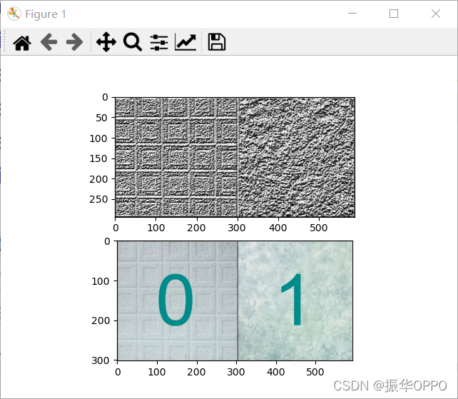
上面一张图是结果LBP算子特征提取后的图片，下面一张图使用SVM进行纹理分类后得到的结果，与预测的左上图纹理相同标为0，与右上图相同标为1。

⭐实验源码+报告⭐

在Linux的各大发行版中，Ubuntu及其衍生版本一直享有对用户友好的美誉。Ubuntu是一个开源操作系统，它的系统和软件可以在官方网站（http://cn.ubuntu.com）免费下载，并且提供了详细的安装方式说明。