读书笔记-深度学习入门之pytorch-第五章（含循环实现手写数字识别）（LSTM、GRU代码详解）

目录

1、RNN优点：（记忆性）

2、循环神经网络结构与原理

3、LSTM（长短时记忆网络）

4、GRU

5、LSTM、RNN、GRU区别

6、收敛性问题

7、循环神经网络Pytorch实现

（1）RNN、LSTM、GRU

（2）LSTM+全连接实现手写数字识别

8、词嵌入（词向量）

9、NGram模型——单词预测

10、序列预测

（1）全连接方法

（2）循环神经网络方法

（3）LSTM方法

  (4)GRU方法

---

1、RNN优点：（记忆性）

RNN对具有序列特性的数据非常有效，它能挖掘数据中的时序信息以及语义信息

2、循环神经网络结构与原理

每一时刻的隐藏层不仅由该时刻的输入层决定，还由上一时刻的隐藏层决定

深层网络结构：

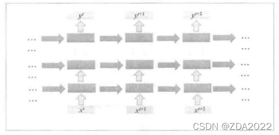
双向循环神经网络：

网络先从序列正方向读取数据，再从反方向读取数据，最后两种输出结果一起形成网络的最终输出

循环神经网络能够很好的解决短时依赖问题，但对于长时依赖问题的效果不是很好 

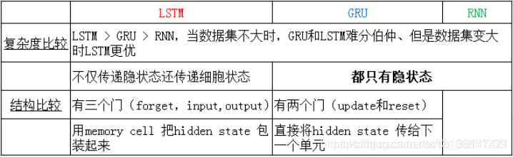
3、LSTM（长短时记忆网络）

 

 4、GRU

5、LSTM、RNN、GRU区别

6、收敛性问题

RNN网络存在收敛性问题，

原因：RNN的误差曲面粗糙不平

解决方法：梯度裁剪

7、循环神经网络Pytorch实现

（1）RNN、LSTM、GRU

LSTM中间比标准RNN多了三个线性变换，多的三个线性变换的权重拼在一起，所以一共是4倍，同理偏置也是4倍。 换句话说，LSTM里面做了4个类似标准RNN所做的运算，所以参数个数是标准RNN的4倍。

GRU:

1. GRU的隐藏状态数量为标准RNN的3倍；
2. 网络的隐藏状态不是 ℎ0和𝑐0h0和c0，而是只有 ℎ0h0；
3. 其余部分和LSTM相同；

from torch import nn

basic_rnn = nn.RNN(input_size=20, hidden_size=50, num_layers=2)
# input_size:输入维度
# hidden_size：输出维度
# num_layers：网络层数
# nonlinearity激活函数
# bias是否使用偏置
# batch_first输入数据的形式，默认是 False，就是这样形式，(seq(num_step), batch, input_dim)，也就是将序列长度放在第一位，batch 放在第二位
# dropout是否应用dropout, 默认不使用，如若使用将其设置成一个0-1的数字即可
# birdirectional是否使用双向的 rnn，默认是 False


lstm = nn.LSTM(input_size=20, hidden_size=50, num_layers=2)

gru = nn.GRU(input_size=20, hidden_size=50, num_layers=2)

（2）LSTM+全连接实现手写数字识别

class Rnn(nn.Module):
    def __init__(self, in_dim=None, hidden_dim=None, n_layer=None):
        super(Rnn, self).__init__()
        self.lstm = nn.LSTM(in_dim, hidden_dim, n_layer, batch_first=True)
        self.classifier = nn.Linear(hidden_dim, 10)

    def forward(self, x):
        x = x.view(x.size(0), 1, -1)  # 构建张量维度

        out, _ = self.lstm(x)
        out = out[:, -1, :]
        out = self.classifier(out)
        return out

 

 

 准确率：97.42%（训练10次）

8、词嵌入（词向量）

词向量的每个维度表示词的某种属性，且词向量夹角越小，表示语义越接近

import torch
from torch import nn
from torch.autograd import Variable

word_to_ix = {'hello': 0, 'world': 1}
embeds = nn.Embedding(2, 5)
hello_idx = torch.LongTensor([word_to_ix['hello']])
hello_idx = Variable(hello_idx)
hello_embed = embeds(hello_idx)
print(hello_embed)

9、NGram模型——单词预测

import torch
import torch.nn as nn
from torch.autograd import Variable
import torch.nn.functional as F
from torch import optim

word_to_ix = {'hello': 0, 'world': 1}
embeds = nn.Embedding(2, 5)
hello_idx = torch.LongTensor([word_to_ix['hello']])
hello_idx = Variable(hello_idx)
hello_embed = embeds(hello_idx)
print(hello_embed)

CONTEXT_SIZE = 2
EMBEDDING_DIM = 10

test_sentence = """When forty winters shall besiege thy brow,
And dig deep trenches in thy beauty's field,
Thy youth's proud livery so gazed on now,
Will be a totter'd weed of small worth held:
Then being asked, where all thy beauty lies,
Where all the treasure of thy lusty days;
To say, within thine own deep sunken eyes,
Were an all-eating shame, and thriftless praise.
How much more praise deserv'd thy beauty's use,
If thou couldst answer 'This fair child of mine
Shall sum my count, and make my old excuse,'
Proving his beauty by succession thine!
This were to be new made when thou art old,
And see thy blood warm when thou feel'st it cold.""".split()

trigram = [((test_sentence[i], test_sentence[i + 1]), test_sentence[i + 2])
           for i in range(len(test_sentence) - 2)]

vocb = set(test_sentence)
word_to_ix = {word: i for i, word in enumerate(vocb)}
idx_to_word = {word_to_ix[word]: word for word in word_to_ix}


class NgramModel(nn.Module):
    def __init__(self, vocb_size, context_size, n_dim):
        super().__init__()
        self.n_word = vocb_size
        self.embedding = nn.Embedding(self.n_word, n_dim)
        self.linear1 = nn.Linear(context_size * n_dim, 128)
        self.linear2 = nn.Linear(128, self.n_word)

    def forward(self, x):
        emb = self.embedding(x)
        emb = emb.view(1, -1)
        out = self.linear1(emb)
        out = F.relu(out)
        out = self.linear2(out)
        log_prob = F.log_softmax(out, 1)
        return log_prob


net = NgramModel(len(vocb), CONTEXT_SIZE, EMBEDDING_DIM)
criterion = nn.CrossEntropyLoss()
optimizer = optim.SGD(net.parameters(), lr=1e-2, weight_decay=1e-5)

epoches = 200

for epoch in range(epoches):
    train_loss = 0
    for word, label in trigram:
        word = Variable(torch.LongTensor([word_to_ix[i] for i in word]))
        label = Variable(torch.LongTensor([word_to_ix[label]]))
        out = net(word)
        loss = criterion(out, label)
        train_loss += loss.item()
        optimizer.zero_grad()
        loss.backward()
        optimizer.step()
    if (epoch + 1) % 20 == 0:
        print('epoch: {}, Loss : {:.6f}'.format(epoch + 1, train_loss / len(trigram)))

net = net.eval()
word, label = trigram[20]
print('input: {}'.format(word))
print('input: {}'.format(label), end="\n\n")

word = Variable(torch.LongTensor([word_to_ix[i] for i in word]))
out = net(word)

pred_label_idx = out.max(1)[1].data[0]
print(pred_label_idx)

predict_word = idx_to_word[int(pred_label_idx)]
print('real word is "{}", predicted word is "{}"'.format(label, predict_word))

 

10、序列预测

（1）全连接方法

# 引入torch相关模块
import torch
from torch import nn, optim
from torch.autograd import Variable
from torch.nn import init

# 引入初始化文件中的相关内容
from seqInit import toTs, cudAvl
from seqInit import input_size
from seqInit import train, real

# 引入画图工具
import numpy as np
import matplotlib.pyplot as plt

# 定义FC模型

class fcModel(nn.Module) :
    def __init__(self, in_dim, hidden_dim, out_dim) :
        super().__init__()
        ly, self.linear = 1, nn.Sequential()
        for hid in hidden_dim :
            layer = nn.Sequential(nn.Linear(in_dim, hid), nn.ReLU(True))
            self.linear.add_module('layer_{}'.format(ly), layer)
            ly, in_dim = ly + 1, hid
        self.linear.add_module('layer_{}'.format(ly), nn.Linear(in_dim, out_dim))
        
        # 使用kaiming_normal初始化模型参数
        self.weightInit(init.kaiming_normal)
    
    def forward(self, x) :
        x = self.linear(x)
        return x
    
    def weightInit(self, func) :
        for name, param in self.named_parameters() :
            if 'weight' in name : func(param)

# 输入为input_size，输出为1，隐藏层设定为3层，分别有[20, 10, 5]的维度
hidden = [20, 10, 5]
fc = cudAvl(fcModel(input_size, hidden, 1))

# 定义损失函数和优化函数
criterion = nn.MSELoss()
optimizer = torch.optim.Adam(fc.parameters(), lr = 1e-2)  



# 制造数据集函数
def create_dataset(dataset, look_back) :
    dataX, dataY = [], []
    for i in range(look_back, len(dataset)) :
        x = dataset[i - look_back: i]
        y = dataset[i]
        dataX.append(x)
        dataY.append(y)
    return np.array(dataX), np.array(dataY)
# 制造训练集
trainX, trainY = create_dataset(train, input_size)
print(trainX.shape, trainY.shape)

# 制造测试集
testX, realY = create_dataset(real, input_size)
print(testX.shape, realY.shape)

# 处理输入
fcx = trainX.reshape(-1, 3)
fcx = torch.from_numpy(fcx)
fcy = trainY.reshape(-1, 1)
fcy = torch.from_numpy(fcy)
print(fcx.shape, fcy.shape)


%%time
# 训练FC模型
frq, sec = 100, 10
loss_set = []
for e in range(1, frq + 1) :
    inputs = cudAvl(Variable(fcx))
    target = cudAvl(Variable(fcy))
    # forward
    outputs = fc(inputs)
    loss = criterion(outputs, target)
    # reset gradients
    optimizer.zero_grad()
    loss.backward()
    optimizer.step()
    # print training infomation
    print_loss = loss.item()
    current = e // sec
    loss_set.append((e, print_loss))
    if e % sec == 0 :
        print_info = 'Epoch[{}/{}], Loss: {:.5f}'.format(current, frq // sec, print_loss)
        print(print_info)

# 作出损失函数变化图像
pltX = np.array([loss[0] for loss in loss_set])
pltY = np.array([loss[1] for loss in loss_set])
plt.title('loss function output curve')
plt.plot(pltX, pltY)
plt.show()


# 测试

px, ry = create_dataset(real, input_size)
px = px.reshape(-1, 3)
ry = ry.reshape(-1, 1)
print(px.shape, ry.shape)
px = torch.from_numpy(px)
px = cudAvl(Variable(px))
py = np.array(fc(px).data)

# 画出实际结果和预测的结果
plt.plot(py, 'r', label='prediction')
plt.plot(ry, 'b', label='real')
plt.legend(loc='best')

 

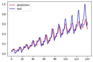
 实际与预测接近

（2）循环神经网络方法

# 引入torch相关模块
import torch
from torch import nn, optim
from torch.autograd import Variable
from torch.nn import init

# 引入初始化文件中的相关内容
from seqInit import toTs, cudAvl
from seqInit import input_size
from seqInit import train, real

# 引入画图工具
import numpy as np
import matplotlib.pyplot as plt

# 定义RNN模型

class rnnModel(nn.Module) :
    def __init__(self, in_dim, hidden_dim, out_dim, layer_num) :
        super().__init__()
        self.rnnLayer = nn.RNN(in_dim, hidden_dim, layer_num)
        self.fcLayer = nn.Linear(hidden_dim, out_dim)
        optim_range = np.sqrt(1.0 / hidden_dim)
        self.weightInit(optim_range)
        
    def forward(self, x) :
        out, _ = self.rnnLayer(x)
        out = out[12:]
        out = self.fcLayer(out)
        return out

    def weightInit(self, gain=1):
        # 使用初始化模型参数
        for name, param in self.named_parameters() :
            if 'rnnLayer.weight' in name :
                init.orthogonal(param, gain)
    
# 输入维度为1，输出维度为1，隐藏层维数为10, 定义rnn层数为2
rnn = cudAvl(rnnModel(1, 10, 1, 2))

# 确定损失函数和优化函数
criterion = nn.MSELoss()
optimizer = optim.Adam(rnn.parameters(), lr = 1e-2)


# 处理输入

def create_dataset(dataset) :
    data = dataset.reshape(-1, 1, 1)
    return torch.from_numpy(data)

trainX = create_dataset(train[:-1])
trainY = create_dataset(train[1:])[12:]
print(trainX.shape, trainY.shape)


# 训练RNN模型
frq, sec = 2000, 200
loss_set = []
for e in range(1, frq + 1) :
    inputs = cudAvl(Variable(trainX))
    target = cudAvl(Variable(trainY))
    # forward
    output = rnn(inputs)
    loss = criterion(output, target)
    # update gradients
    optimizer.zero_grad()
    loss.backward()
    optimizer.step()
    # print training information
    print_loss = loss.item()
    loss_set.append((e, print_loss))
    if e % sec == 0 :
        print('Epoch[{}/{}], loss = {:.5f}'.format(e, frq, print_loss))

# 作损失函数图像
pltX = np.array([loss[0] for loss in loss_set])
pltY = np.array([loss[1] for loss in loss_set])
plt.title('loss function output curve')
plt.plot(pltX, pltY)
plt.show()



# 测试

rnn = rnn.eval()
px = real[:-1].reshape(-1, 1, 1)
px = torch.from_numpy(px)
ry = real[1:].reshape(-1)
varX = cudAvl(Variable(px, volatile=True))
py = rnn(varX).data
py = np.array(py).reshape(-1)
print(px.shape, py.shape, ry.shape)

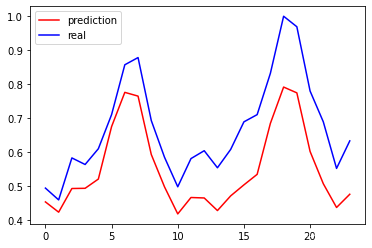
# 画出实际结果和预测的结果
plt.plot(py[-24:], 'r', label='prediction')
plt.plot(ry[-24:], 'b', label='real')
plt.legend(loc='best')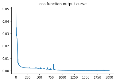

 

（3）LSTM方法

!jupyter nbconvert --to python seqInit.ipynb
import os
os.environ['KMP_DUPLICATE_LIB_OK']='True'

# 引入torch相关模块
import torch
from torch import nn, optim
from torch.autograd import Variable
from torch.nn import init

# 引入初始化文件中的相关内容
from seqInit import toTs, cudAvl
from seqInit import input_size
from seqInit import train, real

# 引入画图工具
import numpy as np
import matplotlib.pyplot as plt

# 定义LSTM模型

class lstmModel(nn.Module) :
    def __init__(self, in_dim, hidden_dim, out_dim, layer_num) :
        super().__init__()
        self.lstmLayer = nn.LSTM(in_dim, hidden_dim, layer_num)
        self.relu = nn.ReLU()
        self.fcLayer = nn.Linear(hidden_dim, out_dim)
        self.weightInit(np.sqrt(1.0 / hidden_dim))
    
    def forward(self, x) :
        out, _ = self.lstmLayer(x)
        out = self.relu(out)
        out = out[12:]
        out = self.fcLayer(out)
        return out
    
    # 初始化权重
    def weightInit(self, gain) :
        for name, param in self.named_parameters():
            if 'lstmLayer.weight' in name :
                init.orthogonal(param)

# 输入维度为1，输出维度为1，隐藏层维数为5, 定义LSTM层数为2
lstm = cudAvl(lstmModel(1, 5, 1, 2))

# 定义损失函数和优化函数

criterion = nn.MSELoss()
optimizer = optim.Adam(lstm.parameters(), lr = 1e-2)

# 处理输入

train = train.reshape(-1, 1, 1)
x = torch.from_numpy(train[:-1])
y = torch.from_numpy(train[1:])[12:]
print(x.shape, y.shape)


%%time

frq, sec = 3500, 350
loss_set = []

for e in range(1, frq + 1) :
    inputs = cudAvl(Variable(x))
    target = cudAvl(Variable(y))
    #forward
    output = lstm(inputs)
    loss = criterion(output, target)
    # update paramters
    optimizer.zero_grad()
    loss.backward()
    optimizer.step()
    #print training information
    print_loss = loss.item()
    loss_set.append((e, print_loss))
    if e % sec == 0 :
        print('Epoch[{}/{}], Loss: {:.5f}'.format(e, frq, print_loss))

# 作出损失函数变化图像
pltX = np.array([loss[0] for loss in loss_set])
pltY = np.array([loss[1] for loss in loss_set])
plt.title('loss function output curve')
plt.plot(pltX, pltY)
plt.show()

lstm = lstm.eval()

# 预测结果并比较

px = real[:-1].reshape(-1, 1, 1)
px = torch.from_numpy(px)
ry = real[1:].reshape(-1)
varX = cudAvl(Variable(px, volatile=True))
py = lstm(varX).data
py = np.array(py).reshape(-1)
print(px.shape, py.shape, ry.shape)

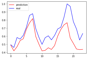
# 画出实际结果和预测的结果
plt.plot(py[-24:], 'r', label='prediction')
plt.plot(ry[-24:], 'b', label='real')
plt.legend(loc='best')

 

 

 

(4)GRU方法

!jupyter nbconvert --to python seqInit.ipynb
import os
os.environ['KMP_DUPLICATE_LIB_OK']='True'

# 引入torch相关模块
import torch
from torch import nn, optim
from torch.autograd import Variable
from torch.nn import init

# 引入初始化文件中的相关内容
from seqInit import toTs, cudAvl
from seqInit import input_size
from seqInit import train, real

# 引入画图工具
import numpy as np
import matplotlib.pyplot as plt

# 定义GRU模型

class gruModel(nn.Module) :
    def __init__(self, in_dim, hidden_dim, out_dim, hidden_layer) :
        super().__init__()
        self.gruLayer = nn.GRU(in_dim, hidden_dim, hidden_layer)
        self.fcLayer = nn.Linear(hidden_dim, out_dim)
    
    def forward(self, x) :
        out, _ = self.gruLayer(x)
        out = out[12:]
        out = self.fcLayer(out)
        return out
        
# 输入维度为1，输出维度为1，隐藏层维数为5, 定义LSTM层数为2
gru = cudAvl(gruModel(1, 5, 1, 2))

# 定义损失函数和优化函数

criterion = nn.MSELoss()
optimizer = optim.Adam(gru.parameters(), lr = 1e-2)

# 处理输入

train = train.reshape(-1, 1, 1)
x = torch.from_numpy(train[:-1])
y = torch.from_numpy(train[1:])[12:]
print(x.shape, y.shape)

%%time
# 训练模型

frq, sec = 4000, 400
loss_set = []

for e in range(1, frq + 1) :
    inputs = cudAvl(Variable(x))
    target = cudAvl(Variable(y))
    #forward
    output = gru(inputs)
    loss = criterion(output, target)
    # update paramters
    optimizer.zero_grad()
    loss.backward()
    optimizer.step()
    #print training information
    print_loss = loss.item()
    loss_set.append((e, print_loss))
    if e % sec == 0 :
        print('Epoch[{}/{}], Loss: {:.5f}'.format(e, frq, print_loss))

# 作出损失函数变化图像
pltX = np.array([loss[0] for loss in loss_set])
pltY = np.array([loss[1] for loss in loss_set])
plt.title('loss function output curve')
plt.plot(pltX, pltY)
plt.show()


gru = gru.eval()

# 预测结果并比较

px = real[:-1].reshape(-1, 1, 1)
px = torch.from_numpy(px)
ry = real[1:].reshape(-1)
varX = cudAvl(Variable(px, volatile=True))
py = gru(varX).data
py = np.array(py).reshape(-1)
print(px.shape, py.shape, ry.shape)

# 画出实际结果和预测的结果
plt.plot(py[-24:], 'r', label='prediction')
plt.plot(ry[-24:], 'b', label='real')
plt.legend(loc='best')