【LSTM】从Kaggle股价预测问题了解LSTM

模型效果：

1 数据集

参考了kaggle的一个notebook，它只考虑了input_dim是1的情况，我这里改成了input_dim=2，别的内容比较相似。

notebook：https://www.kaggle.com/code/taronzakaryan/predicting-stock-price-using-lstm-model-pytorch

数据集：https://www.kaggle.com/datasets/borismarjanovic/price-volume-data-for-all-us-stocks-etfs

Here I provide the full historical daily price and volume data for all US-based stocks and ETFs trading on the NYSE, NASDAQ, and NYSE MKT.

在这里，我提供了在纽约证券交易所、纳斯达克和纽约证券交易所MKT交易的所有美国股票和ETF的完整的历史每日价格和交易量数据。ETF(Exchange Traded Fund)是交易所交易基金，是一种可以在证券交易所上市交易的开放式基金。

The data (last updated 11/10/2017) is presented in CSV format as follows: Date, Open, High, Low, Close, Volume, OpenInt. Note that prices have been adjusted for dividends and splits.

数据(最后更新日期为2017年10月11日)以CSV格式呈现如下：日期，开盘价，最高价，最低价，收盘价，成交量，OpenInt。请注意，价格已根据股息和分拆进行了调整。

OpenInt通常指期货或期权合约的未平仓合约数，它表示当前尚未平仓的合约数量。

数据示例：

Date	Open	High	Low	Close	Volume	OpenInt
2010-07-21	24.333	24.333	23.946	23.946	43321	0
2010-07-22	24.644	24.644	24.362	24.487	18031	0
2010-07-23	24.759	24.759	24.314	24.507	8897	0
2010-07-26	24.624	24.624	24.449	24.595	19443	0
2010-07-27	24.477	24.517	24.431	24.517	8456	0

如果希望看一下数据集趋势的话，以收盘价Close为例：

def stocks_data(companies, dates):
    """
    将多个commpanies的Stock收盘价合并在一起，得到一个大的DataFrame
    :param companies:
    :param dates:
    :return:
    """

    # 选取dates包含的日期列
    df = pd.DataFrame(index=dates)

    # 对每个company的Stock交易数据，以'Date'作为索引列，将Date解析为日期格式，且指定Close收盘价作为读取的数据列
    # 读到缺失数据是转化为nan
    for company in companies:
        df_temp = pd.read_csv(
            "Data/Stocks/{}.us.txt".format(company),
            index_col='Date',
            parse_dates=True,
            usecols=['Date', 'Close'],
            na_values=['nan']
        )
        df_temp = df_temp.rename(columns={'Close': company})
        df = df.join(df_temp)
    return df


dates = pd.date_range('2015-01-02', '2016-12-31', freq='B') # Business Day，工作日
companies = ['goog', 'ibm', 'aapl']
df = stocks_data(companies, dates)
# 在数据中出现缺失值时，函数会在该位置之前的最后一个非缺失值和该位置之后的最近一个非缺失值之间进行线性插值（即‘pad’方法）
df.fillna(method='pad')
df.plot(figsize=(10, 6), subplots=True)
plt.show()

再来看一眼IBM的，也是我们的预测目标：

# ------------ 展示一下IBM在2010-01-02到2017-10-11的股价走向 ----------------

dates = pd.date_range('2010-01-02', '2017-10-11', freq='B')
df1 = pd.DataFrame(index=dates)
df_ibm = pd.read_csv("Data/Stocks/ibm.us.txt", parse_dates=True, index_col=0)
df_ibm = df1.join(df_ibm)
df_ibm[['Close']].plot(figsize=(15, 6))
plt.ylabel("stock_price")
plt.title("IBM Stock")
plt.show()

数据情况：还是有缺失值的，需要fillna一下

DatetimeIndex: 2028 entries, 2010-01-04 to 2017-10-11
Freq: B
Data columns (total 1 columns):
 #   Column  Non-Null Count  Dtype  
---  ------  --------------  -----  
 0   Close   1958 non-null   float64
dtypes: float64(1)
memory usage: 96.2 KB

2 数据预处理

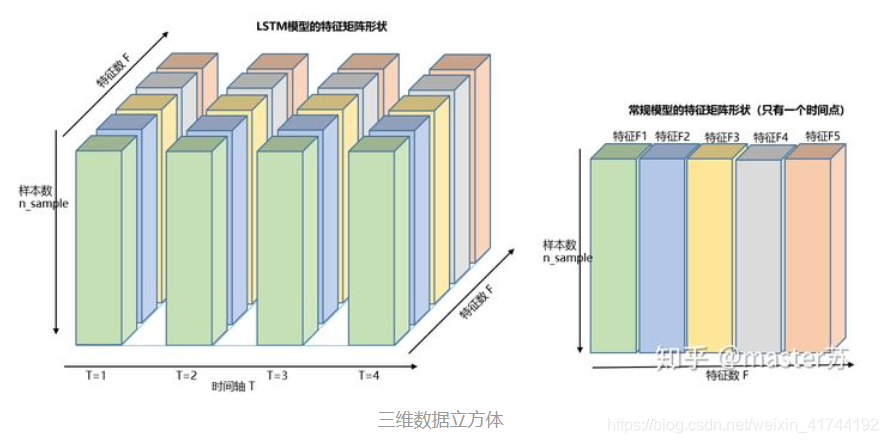
为了简单展示时间序列预测问题的三个维度$(batch\_size,seq\_size,input\_size)$，我们采用very very brute force的方式，没有划分batch，把整个X_train当成一个batch_size=1574的大大batch。

seq_size设置为59，即回看过去的59天数据，input_size设置为2，考虑开盘价Open与收盘价Close，预测当天收盘价Close。

# 将缺失值使用前一个非缺失值填充
df_ibm = df_ibm.fillna(method='ffill')
# 进行归一化处理，放缩到(-1, 1)范围内
scaler = MinMaxScaler(feature_range=(-1, 1))
df_ibm['Close'] = scaler.fit_transform(df_ibm['Close'].values.reshape(-1, 1))
df_ibm['Open'] = scaler.fit_transform(df_ibm['Open'].values.reshape(-1, 1))

切一下训练集和测试集：

# function to create train, test data given stock data and sequence length
def load_data(stock, look_back):
    data_raw = stock.values  # 转换为numpy数组
    data = []

    # 通过滑动的窗口生成所有可能的长度为look_back的序列
    for index in range(len(data_raw) - look_back):
        data.append(data_raw[index: index + look_back])

    # 将list转换为一个numpy数组~
    data = np.array(data)
    test_set_size = int(np.round(0.2 * data.shape[0]))
    train_set_size = data.shape[0] - test_set_size

    # 切得训练集
    x_train = data[:train_set_size, :-1, :]
    y_train = data[:train_set_size, -1, -1:]

    # 测试集
    x_test = data[train_set_size:, :-1]
    y_test = data[train_set_size:, -1, -1:]

    return [x_train, y_train, x_test, y_test]


look_back = 60  # 序列长度，预测时回看多少个日子的股价

# x_train.shape =  (1574, 59, 2)
# y_train.shape =  (1574, 1)
# x_test.shape =  (394, 59, 2)
# y_test.shape =  (394, 1)
x_train, y_train, x_test, y_test = load_data(df_ibm, look_back)

为了适应后面LSTM的输入要求操作，调换一下X的数据维度，原来是(batch, seq_size, input_dim)，现在变为(seq_size, batch, input_dim)。

# x_train.shape =  (59, 1574, 2)
# y_train.shape =  (1574, 1)
# x_test.shape =  (59, 394, 2)
# y_test.shape =  (394, 1)
x_train = x_train.transpose((1, 0, 2))
x_test = x_test.transpose((1, 0, 2))

转换为Pytorch张量：

# 转换为pytorch的张量
x_train = torch.from_numpy(x_train).type(torch.Tensor)
x_test = torch.from_numpy(x_test).type(torch.Tensor)
y_train = torch.from_numpy(y_train).type(torch.Tensor)
y_test = torch.from_numpy(y_test).type(torch.Tensor)

数据输入结构示意

3 LSTM

这部分LSTM的知识参考了这个blog，先给出实现然后再进行解释。

3.1 LSTM单元

3.2 定义LSTM网络

import torch
import torch.nn as nn


class LSTM(nn.Module):
    def __init__(self, input_dim, hidden_dim, num_layers, output_dim):
        super(LSTM, self).__init__()

        # 隐层单元数目
        self.hidden_dim = hidden_dim

        # 隐层数目
        self.num_layers = num_layers

        # batch_first=True
        # 使 输入输出 张量的维度为：(batch_dim, seq_dim, feature_dim)
        self.lstm = nn.LSTM(input_dim, hidden_dim, num_layers)

        # 全连接层
        self.fc = nn.Linear(hidden_dim, output_dim)

    def forward(self, x):
        # 用0初始化隐层状态
        h0 = torch.zeros(self.num_layers, x.size(1), self.hidden_dim).requires_grad_()

        # 用0初始化细胞状态
        c0 = torch.zeros(self.num_layers, x.size(1), self.hidden_dim).requires_grad_()

        # 我们需要detach()以进行经过时间截断的BPTT
        # 如果不这样做，我们会一直反向传播到起点
        out, (hn, cn) = self.lstm(x, (h0.detach(), c0.detach()))

        # 最后一个时间步的隐藏状态
        out = self.fc(out[-1, :, :])
        return out

3.3 Pytorch中的LSTM

self.lstm = nn.LSTM(input_dim, hidden_dim, num_layers, batch_first=True)

class torch.nn.LSTM(*args, **kwargs)
参数有：
    input_size：x的特征维度
    hidden_size：隐藏层的特征维度
    num_layers：lstm隐层的层数，默认为1
    bias：False则bih=0和bhh=0. 默认为True
    batch_first：默认为False，True则输入输出的数据格式为 (batch, seq, feature)
    dropout：除最后一层，每一层的输出都进行dropout，默认为: 0

设置num_layer=2意味着将两个LSTM堆叠在一起形成一个堆叠的 LSTM，第二个 LSTM 接收第一个 LSTM 的输出并计算最终结果。

像这样子，是纵向的两层。而不是横向的时间步传播。

调用：

out, (hn, cn) = self.lstm(x, (h0.detach(), c0.detach()))

参数

一层有4个参数，两层共有8个参数。

• LSTM.weight_ih_l[k] – 学习得到的第k层的 input-hidden 权重$ (W_ii|W_if|W_ig|W_io)$，当k=0 时形状为 (4hidden_size, input_size) 。 否则，形状为 (4hidden_size, num_directions * hidden_size)
• LSTM.weight_hh_l[k] –学习得到的第k层的 hidden -hidden 权重$(W_{h}i|W_{h}f|W_{h}g|W_{h}o)$, 想形状为 (4hidden_size, hidden_size)。如果 Proj_size > 0，则形状为 (4hidden_size, proj_size)
• LSTM.bias_ih_l[k] – 学习得到的第k层的input-hidden 的偏置 $(b_{i}i|b_{i}f|b_{i}g|b_{i}o)$, 形状为 (4hidden_size)
• LSTM.bias_hh_l[k] – 学习得到的第k层的hidden -hidden 的偏置 $ (b_hi|b_hf|b_hg|b_ho)$, 形状为 (4*hidden_size)

结合上面这个图来看就是说：所有与$x$相关的$W$，即$W_{xf}、W_{xi}、W_{xg}、W_{xo}$作为一个参数$W_x$；所有与$h$相关的$W$作为一个参数$W_h$；所有与$x$相关的$b$作为一个参数；所有与$h$相关的$b$作为一个参数。一层一共有4个参数。

可以理解成一梭子算完线性乘积，然后再拆成4个部分做上面图中的操作。

第一层参数：
Wx：torch.Size([128, 2])
Wh：torch.Size([128, 32])
bx：torch.Size([128])
bh：torch.Size([128])

Wx：torch.Size([128, 32])
Wh：torch.Size([128, 32])
bx：torch.Size([128])
bh：torch.Size([128])

直观理解

输入

LSTM的默认输入格式为：input(seq_len, batch, input_size),

如果设置了batch_first=True，则输入格式为input(batch, seq_len, input_size)，这种格式更好理解。

注：batch_first的设置不会影响h和c的形状，因为内部计算时已经对input的格式进行了转换。

LSTM的另外两个输入是 h0 和 c0，可以理解成网络的初始化参数，用随机数生成即可。

h0(num_layers, batch, hidden_size)
c0(num_layers, batch, hidden_size)
参数：
    num_layers：隐藏层数
    batch：输入数据的batch (因为每个batch会有不同的隐状态嘛
    hidden_size：隐藏层神经元个数

输出

LSTM的输出是一个tuple，如下：

• output: 最后一个状态的隐藏层的神经元输出
• hn：最后一个状态的隐含层的状态值
• cn：最后一个状态的隐含层的记忆细胞值

output的默认维度是：

output(seq_len, batch, hidden_size)
ht(num_layers, batch, hidden_size)
ct(num_layers, batch, hidden_size)

训练过程

num_epochs = 100
hist = np.zeros(num_epochs)

# Number of steps to unroll
seq_dim = look_back - 1

for t in range(num_epochs):
    # 初始化隐藏层状态
    # Don't do this if you want your LSTM to be stateful
    # model.hidden = model.init_hidden()
    
    # 清空这个epoch的梯度
    optimizer.zero_grad()

    # 前向传递
    y_train_pred = model(x_train)

    # 计算损失
    loss = loss_fn(y_train_pred, y_train)
    if t % 10 == 0 and t != 0:
        print("Epoch ", t, "MSE: ", loss.item())
    hist[t] = loss.item()

    # 反向传播
    loss.backward()

    # 更新参数
    optimizer.step()

完整代码

LSTM.py

import torch
import torch.nn as nn


class LSTM(nn.Module):
    def __init__(self, input_dim, hidden_dim, num_layers, output_dim):
        super(LSTM, self).__init__()

        # 隐层单元数目
        self.hidden_dim = hidden_dim

        # 隐层数目
        self.num_layers = num_layers

        # batch_first=True
        # 使 输入输出 张量的维度为：(batch_dim, seq_dim, feature_dim)
        self.lstm = nn.LSTM(input_dim, hidden_dim, num_layers)

        # 全连接层
        self.fc = nn.Linear(hidden_dim, output_dim)

    def forward(self, x):
        # 用0初始化隐层状态
        h0 = torch.zeros(self.num_layers, x.size(1), self.hidden_dim).requires_grad_()

        # 用0初始化细胞状态
        c0 = torch.zeros(self.num_layers, x.size(1), self.hidden_dim).requires_grad_()

        # 我们需要detach()以进行经过时间截断的BPTT
        # 如果不这样做，我们会一直反向传播到起点
        out, (hn, cn) = self.lstm(x, (h0.detach(), c0.detach()))

        # 最后一个时间步的隐藏状态
        out = self.fc(out[-1, :, :])
        return out

main.py

import math

import numpy as np
import pandas as pd
from pylab import mpl
import matplotlib.pyplot as plt
from sklearn.metrics import mean_squared_error

plt.style.use('seaborn')
mpl.rcParams['font.family'] = 'serif'

from sklearn.preprocessing import MinMaxScaler
import torch

from LSTM import LSTM


def stocks_data(companies, dates):
    """
    将多个commpanies的Stock收盘价合并在一起，得到一个大的DataFrame
    :param companies:
    :param dates:
    :return:
    """

    # 选取dates包含的日期列
    df = pd.DataFrame(index=dates)

    # 对每个company的Stock交易数据，以'Date'作为索引列，将Date解析为日期格式，且指定Close收盘价作为读取的数据列
    # 读到缺失数据是转化为nan
    for company in companies:
        df_temp = pd.read_csv(
            "Data/Stocks/{}.us.txt".format(company),
            index_col='Date',
            parse_dates=True,
            usecols=['Date', 'Close'],
            na_values=['nan']
        )
        df_temp = df_temp.rename(columns={'Close': company})
        df = df.join(df_temp)
    return df


# ------------ 展示一下google，IBM，aapl的股价走向 ---------------------------

dates = pd.date_range('2015-01-02', '2016-12-31', freq='B')  # B表示工作日Business Day
companies = ['goog', 'ibm', 'aapl']
df = stocks_data(companies, dates)
# 在数据中出现缺失值时，函数会在该位置之前的最后一个非缺失值和该位置之后的最近一个非缺失值之间进行线性插值（即‘pad’方法）
df.fillna(method='pad')
df.plot(figsize=(10, 6), subplots=True)
plt.show()

# ------------ 展示一下IBM在2010-01-02到2017-10-11的股价走向 ----------------

dates = pd.date_range('2010-01-02', '2017-10-11', freq='B')
df1 = pd.DataFrame(index=dates)
df_ibm = pd.read_csv("Data/Stocks/ibm.us.txt", parse_dates=True, index_col=0)
df_ibm = df1.join(df_ibm)
df_ibm[['Close']].plot(figsize=(15, 6))
plt.ylabel("stock_price")
plt.title("IBM Stock")
plt.show()

# ------------ 简单Info ---------------------------------------------------

df_ibm = df_ibm[['Open', 'Close']]
# df_ibm.info()

# ------------ 数据预处理 --------------------------------------------------

# 将缺失值使用前一个非缺失值填充
df_ibm = df_ibm.fillna(method='ffill')
# 进行归一化处理，放缩到(-1, 1)范围内
scaler = MinMaxScaler(feature_range=(-1, 1))
df_ibm['Close'] = scaler.fit_transform(df_ibm['Close'].values.reshape(-1, 1))
df_ibm['Open'] = scaler.fit_transform(df_ibm['Open'].values.reshape(-1, 1))


# ------------ 准备训练集测试集  ---------------------------------------------


# function to create train, test data given stock data and sequence length
def load_data(stock, look_back):
    data_raw = stock.values  # 转换为numpy数组
    data = []

    # 通过滑动的窗口生成所有可能的长度为look_back的序列
    for index in range(len(data_raw) - look_back):
        data.append(data_raw[index: index + look_back])

    # 将list转换为一个numpy数组~
    data = np.array(data)
    test_set_size = int(np.round(0.2 * data.shape[0]))
    train_set_size = data.shape[0] - test_set_size

    # 切得训练集
    x_train = data[:train_set_size, :-1, :]
    y_train = data[:train_set_size, -1, -1:]

    # 测试集
    x_test = data[train_set_size:, :-1]
    y_test = data[train_set_size:, -1, -1:]

    return [x_train, y_train, x_test, y_test]


look_back = 60  # 序列长度，预测时回看多少个日子的股价

# x_train.shape =  (1574, 59, 2)
# y_train.shape =  (1574, 1)
# x_test.shape =  (394, 59, 2)
# y_test.shape =  (394, 1)
x_train, y_train, x_test, y_test = load_data(df_ibm, look_back)

# x_train.shape =  (59, 1574, 2)
# y_train.shape =  (1574, 1)
# x_test.shape =  (59, 394, 2)
# y_test.shape =  (394, 1)
x_train = x_train.transpose((1, 0, 2))
x_test = x_test.transpose((1, 0, 2))

# 转换为pytorch的张量
x_train = torch.from_numpy(x_train).type(torch.Tensor)
x_test = torch.from_numpy(x_test).type(torch.Tensor)
y_train = torch.from_numpy(y_train).type(torch.Tensor)
y_test = torch.from_numpy(y_test).type(torch.Tensor)

#  ------------------------------------ 新建一个model --------------------------

input_dim = 2
hidden_dim = 32
num_layers = 2
output_dim = 1

model = LSTM(input_dim=input_dim, hidden_dim=hidden_dim, output_dim=output_dim, num_layers=num_layers)

loss_fn = torch.nn.MSELoss()
optimizer = torch.optim.Adam(model.parameters(), lr=0.01)
print(model)
print(len(list(model.parameters())))
for i in range(len(list(model.parameters()))):
    print(list(model.parameters())[i].size())

# ------------------------------------- 训练过程 ----------------------------

num_epochs = 100
hist = np.zeros(num_epochs)

# Number of steps to unroll
seq_dim = look_back - 1

for t in range(num_epochs):
    # 初始化隐藏层状态
    # stateful: 要求隐状态在不同的batch之间保持不变
    # Don't do this if you want your LSTM to be stateful
    # model.hidden = model.init_hidden()

    # 清空这个epoch的梯度
    optimizer.zero_grad()

    # 前向传递
    y_train_pred = model(x_train)

    # 计算损失
    loss = loss_fn(y_train_pred, y_train)
    if t % 10 == 0 and t != 0:
        print("Epoch ", t, "MSE: ", loss.item())
    hist[t] = loss.item()

    # 反向传播
    loss.backward()

    # 更新参数
    optimizer.step()

plt.plot(hist, label="Training loss")
plt.legend()
plt.show()

# ------------------------------- 预测 ----------------------------------------------=

# make predictions
y_test_pred = model(x_test)

# invert predictions
y_train_pred = scaler.inverse_transform(y_train_pred.detach().numpy())
y_train = scaler.inverse_transform(y_train.detach().numpy())
y_test_pred = scaler.inverse_transform(y_test_pred.detach().numpy())
y_test = scaler.inverse_transform(y_test.detach().numpy())

# calculate root mean squared error
trainScore = math.sqrt(mean_squared_error(y_train[:, 0], y_train_pred[:, 0]))
print('Train Score: %.2f RMSE' % (trainScore))
testScore = math.sqrt(mean_squared_error(y_test[:, 0], y_test_pred[:, 0]))
print('Test Score: %.2f RMSE' % (testScore))

figure, axes = plt.subplots(figsize=(15, 6))
axes.xaxis_date()

axes.plot(df_ibm[len(df_ibm) - len(y_test):].index, y_test, color='red', label='Real IBM Stock Price')
axes.plot(df_ibm[len(df_ibm) - len(y_test):].index, y_test_pred, color='blue', label='Predicted IBM Stock Price')
# axes.xticks(np.arange(0,394,50))
plt.title('IBM Stock Price Prediction')
plt.xlabel('Time')
plt.ylabel('IBM Stock Price')
plt.legend()
plt.savefig('ibm_pred.png')
plt.show()

测试结果：还是有点overfit的，训练集结果要比测试集好很多，不过也只是一个二层的网络，不强求了。