计算机视觉（二）：局部图像描述子

一、序

局部图像描述子主要是为了寻找图像间的对应点和对应区域。以下内容将出现两种用于图像匹配的局部描述子算法。
特征匹配的基本流程：

1. 根据特定准则，提取图像中的特征点
2. 提取特征点周围的图像块，构造特征描述符
3. 通过特征描述符对比，实现特征匹配
   特征点必须具有不变性

特征可以分为以下几类：

1. 角点：Harris算子，SUSAN算子。FSAT算子
2. 梯度特征点：SIFT、SURF、GLOH、ASIFT、PSIFT算子
3. 边缘特征（线性）：Canny算子、Marr算子
4. 纹理特征：灰度共生矩阵，小波Gabor算子
5. 快速特征匹配的基本策略：以图像中稳定角点的领域训练特征分类器，为输入图像的特征分类

1、角点（corner points）

局部窗口沿各方向移动，均产生明显变化的点
图像局部曲率突变的点

经典的角点检测算法
Harris角点检测
CSS角点检测

2. 如何判断是否是好的角点检测算法

• 检测出图像中“真实的”角点
• 准确的定位性能
• 很高的稳定性
• 具有对噪声的鲁棒性
• 具有较高的计算效率

二、Harris角点检测器

1、基本思想

从图像局部的小窗口观察图像特征，利用角点定义判断，如下图

如果在平坦区域：那么超任意方向移动，都无灰度变化
如果在边缘处移动：沿着边缘方向移动，无灰度变化
在角点处：沿任意方向移动，有明显的灰度变化

2、数学表达

将图像窗口平移==[u,v]产生灰度变化E(u,v)==

我们可以利用泰勒展开来获得上图式子中的E和I
窗口函数的两种表示：

对于局部微小的移动量[u,v]，我们可以获得以下近似值

M是由图像的导数求得的2X2的矩阵。
所以窗口移动导致的图像变化量其实就是对对称矩阵M的特征值分析，通过两个特征值的大小我们可以对图像点进行分类：

当两个特征值都很小时，图像窗口在所有方向上移动都无明显灰度变化
我们可以定义一个角点响应函数R：

我们将上面的区域划分换一种划分方式，则为：

我们可以看到：
在角点时：R为大叔之正数
在边缘点时：R为大数值负数
在平坦区时：R为小数值

3、角点计算流程

1. 对角点响应函数R进行阈值处理
   R>threshold
2. 提取R的局部极大值

为了消除参数k的影响，也可以采用商来计算响应：

4、算法实现

4.1 角点响应函数

from scipy.ndimage import filters


def compute_harris_response(im,sigma=3):
    """ Compute the Harris corner detector response function 
        for each pixel in a graylevel image. """
    
    
    imx = zeros(im.shape)
    filters.gaussian_filter(im, (sigma,sigma), (0,1), imx)
    imy = zeros(im.shape)
    filters.gaussian_filter(im, (sigma,sigma), (1,0), imy)
    
    Wxx = filters.gaussian_filter(imx*imx,sigma)
    Wxy = filters.gaussian_filter(imx*imy,sigma)
    Wyy = filters.gaussian_filter(imy*imy,sigma)
    
    Wdet = Wxx*Wyy - Wxy**2
    Wtr = Wxx + Wyy
    
    return Wdet / (Wtr*Wtr)

4.2 筛选角点

def get_harris_points(harrisim,min_dist=10,threshold=0.1):
    
    # find top corner candidates above a threshold
    corner_threshold = harrisim.max() * threshold
    harrisim_t = (harrisim > corner_threshold) * 1
    
    # get coordinates of candidates
    coords = array(harrisim_t.nonzero()).T
    
    # ...and their values
    candidate_values = [harrisim[c[0],c[1]] for c in coords]
    
    # sort candidates
    index = argsort(candidate_values)
    
    # store allowed point locations in array
    allowed_locations = zeros(harrisim.shape)
    allowed_locations[min_dist:-min_dist,min_dist:-min_dist] = 1
    
    # select the best points taking min_distance into account
    filtered_coords = []
    for i in index:
        if allowed_locations[coords[i,0],coords[i,1]] == 1:
            filtered_coords.append(coords[i])
            allowed_locations[(coords[i,0]-min_dist):(coords[i,0]+min_dist), 
                        (coords[i,1]-min_dist):(coords[i,1]+min_dist)] = 0
    
    return filtered_coords

4.3 显示角点

def plot_harris_points(image,filtered_coords):
    
    figure()
    gray()
    imshow(image)
    plot([p[1] for p in filtered_coords],
                [p[0] for p in filtered_coords],'*')
    axis('off')
    show()

4.4 结果显示

原图：

5. 寻找对应点

5.1 兴趣点描述子

分配给兴趣点的一个向量，描述该点附近的图像的表观信息。描述子约到，寻找到的对应点越好。描述子通常是由周围图像像素块的灰度值，以及用于比较归一互相关矩阵构成的。

5.1.1 获取图像像素块，并使用归一化的互相关矩阵进行比较

def get_descriptors(image,filtered_coords,wid=5):
    
    desc = []
    for coords in filtered_coords:
        patch = image[coords[0]-wid:coords[0]+wid+1,
                            coords[1]-wid:coords[1]+wid+1].flatten()
        desc.append(patch)
    
    return desc

def match(desc1,desc2,threshold=0.5):
    
    n = len(desc1[0])
    
    # pair-wise distances
    d = -ones((len(desc1),len(desc2)))
    for i in range(len(desc1)):
        for j in range(len(desc2)):
            d1 = (desc1[i] - mean(desc1[i])) / std(desc1[i])
            d2 = (desc2[j] - mean(desc2[j])) / std(desc2[j])
            ncc_value = sum(d1 * d2) / (n-1) 
            if ncc_value > threshold:
                d[i,j] = ncc_value
            
    ndx = argsort(-d)
    matchscores = ndx[:,0]
    
    return matchscores

def match_twosided(desc1,desc2,threshold=0.5):
    
    matches_12 = match(desc1,desc2,threshold)
    matches_21 = match(desc2,desc1,threshold)
    
    ndx_12 = where(matches_12 >= 0)[0]
    
    # remove matches that are not symmetric
    for n in ndx_12:
        if matches_21[matches_12[n]] != n:
            matches_12[n] = -1
    
    return matches_12

匹配点可视化

def appendimages(im1,im2):
    
    # select the image with the fewest rows and fill in enough empty rows
    rows1 = im1.shape[0]    
    rows2 = im2.shape[0]
    
    if rows1 < rows2:
        im1 = concatenate((im1,zeros((rows2-rows1,im1.shape[1]))),axis=0)
    elif rows1 > rows2:
        im2 = concatenate((im2,zeros((rows1-rows2,im2.shape[1]))),axis=0)
    # if none of these cases they are equal, no filling needed.
    
    return concatenate((im1,im2), axis=1)
def plot_matches(im1,im2,locs1,locs2,matchscores,show_below=True):
    
    im3 = appendimages(im1,im2)
    if show_below:
        im3 = vstack((im3,im3))
    
    imshow(im3)
    
    cols1 = im1.shape[1]
    for i,m in enumerate(matchscores):
        if m>0:
            plot([locs1[i][1],locs2[m][1]+cols1],[locs1[i][0],locs2[m][0]],'c')
    axis('off')

结果显示

三、SIFT算法

1、产生

David G.Lowe教授总结了基于特征不变技术的检测方法，在图像尺度空间基础上，提出对图像缩放、旋转保存不变性的图像局部特征描述算子–SIFT，即尺度不变特征变换。
SIFT算法可以解决以下问题：

• 目标的旋转、缩放、平移
• 图像仿射/投影变换
• 弱光照影响
• 部分目标遮挡
• 杂物场景
• 噪声

2、了解

实质可以归为在不同尺度空间商查找特征点（关键点）的问题

流程如下：

1. 提取关键点
2. 对关键点附加详细信息（局部特征），即描述符
3. 通过特征点（附带上特征向量的关键点）的两两比较找出相互匹配的若干对特征点，建立对应关系

SIFT要查找的点是一些十分突出的点，不会因光照、尺度、旋转等因素的改变而消失 ，比如：角点、边缘点、暗区域的点以及亮区域的暗点。也就是说SIFT希望选出在尺度、旋转、亮度都具有不变性的点

主要思想是通过对原始图像进行尺度变换，获得图像多尺度下的空间表示。从而实现边缘、角点检测和不同分辨率上的特征提取，以满足特征点的尺度不变性。尺度越大图像越模糊。

2.1 兴趣点

SIFT特征使用高斯差分函数来定位兴趣点：

DoG高斯差分金字塔：对应DOG算子，需构建DOG金字塔
通过高斯差分图像看出图像上的像素值变化情况。如果没有变化，也就没有特征。特征必须是变化尽可能多的点。DOG图像描绘的是目标轮廓。

DOG的局部极值点：特征点是由DOG空间得局部极值点组成的。每一个像素点要和它所有的相邻点比较，看其是否比它的图像域和尺度域的相邻点大或者小。

中间的监测点和它同尺度的8个相邻点和上下相邻尺度对应的9×2个点共26个点比较，以确保在尺度空间和二维图像空间都检测到极值点。

去除边缘响应DOG函数在图像边缘有较强的边缘响应。DOG函数的峰值点在边缘方向有较大的主曲率，在垂直边缘的方向有较小的主曲率。主曲率可以通过计算在该点位置尺度的2×2的Hessian矩阵得到。

2.2 描述子

为了实现旋转不变性，基于每个点周围图像梯度的方向和大小。SIFT描述子又引入参考方向。SIFT描述子使用主方向描述参考方向。

2.3 检测兴趣点

使用开源工具包VLFeat提供的二进制文件来计算图像的SIFT特征。代码如下：

def process_image(imagename,resultname,params="--edge-thresh 10 --peak-thresh 5"):

    if imagename[-3:] != 'pgm':
        # create a pgm file
        im = Image.open(imagename).convert('L')
        im.save('tmp.pgm')
        imagename = 'tmp.pgm'

    cmmd = str("sift "+imagename+" --output="+resultname+
                " "+params)
    os.system(cmmd)
    print ('processed', imagename, 'to', resultname)
    
#读取特征数值到数值
def read_features_from_file(filename):
    
    f = loadtxt(filename)
    return f[:,:4],f[:,4:]

#输出结构保存到特征图片
def write_features_to_file(filename,locs,desc):
    savetxt(filename,hstack((locs,desc)))


#可视化
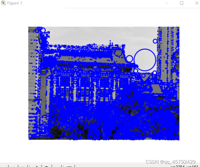
def plot_features(im,locs,circle=False):

    def draw_circle(c,r):
        t = arange(0,1.01,.01)*2*pi
        x = r*cos(t) + c[0]
        y = r*sin(t) + c[1]
        plot(x,y,'b',linewidth=2)

    imshow(im)
    if circle:
        for p in locs:
            draw_circle(p[:2],p[2]) 
    else:
        plot(locs[:,0],locs[:,1],'ob')
    axis('off')

2.4 匹配描述子

一图像中的特征匹配到另一幅图像的特征，使用两个特征距离和两个最匹配特征距离的比率。相对于图像的其他特征，该准则保证能够找到足够相似的唯一特征。能够降低错误的匹配数。

代码：

def match(desc1,desc2):
    
    desc1 = array([d/linalg.norm(d) for d in desc1])
    desc2 = array([d/linalg.norm(d) for d in desc2])
    
    dist_ratio = 0.6
    desc1_size = desc1.shape
    
    matchscores = zeros((desc1_size[0]),'int')
    desc2t = desc2.T # precompute matrix transpose
    for i in range(desc1_size[0]):
        dotprods = dot(desc1[i,:],desc2t) # vector of dot products
        dotprods = 0.9999*dotprods
        # inverse cosine and sort, return index for features in second image
        indx = argsort(arccos(dotprods))
        
        # check if nearest neighbor has angle less than dist_ratio times 2nd
        if arccos(dotprods)[indx[0]] < dist_ratio * arccos(dotprods)[indx[1]]:
            matchscores[i] = int(indx[0])
    
    return matchscores

该函数使用描述子向量间的家教作为距离度量。但是我们需要将描述子向量归一化到单位长度。因为匹配是单向的，所以我们可以先计算第二幅图兴趣点描述子向量的装置矩阵。

为了增加匹配的稳健性，我们可以再反过来执行一次该步骤，从第二幅图象中的特征向第一幅图像中的特征匹配。最后，我们保留同时满足这两种匹配准则的对应。代码如下：

def match_twosided(desc1,desc2):
    
    matches_12 = match(desc1,desc2)
    matches_21 = match(desc2,desc1)
    
    ndx_12 = matches_12.nonzero()[0]
    
    # remove matches that are not symmetric
    for n in ndx_12:
        if matches_21[int(matches_12[n])] != n:
            matches_12[n] = 0
    
    return matches_12

四、匹配地理标记图像

1、下载地理标记图像

从Panoramio下载图像，其提供了一个API接口

import os
import urllib, urlparse 
import json

# query for images
url = 'http://www.panoramio.com/map/get_panoramas.php?order=popularity&set=public&from=0&to=20&minx=-77.037564&miny=38.896662&maxx=-77.035564&maxy=38.898662&size=medium'
c = urllib.urlopen(url)

# get the urls of individual images from JSON
j = json.loads(c.read()) 
imurls = []
for im in j['photos']:
    imurls.append(im['photo_file_url'])

# download images
for url in imurls:
    image = urllib.URLopener()
    image.retrieve(url, os.path.basename(urlparse.urlparse(url).path)) 
    print 'downloading:', url

2、使用局部描述子匹配

对图像进行SIFT特征处理后，将特征保存，使用下列代码进行逐个匹配

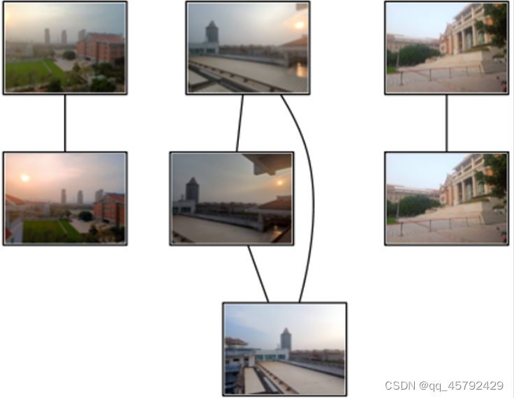
3、可视化连接的图像

使用pydot工具包进行可视化连接。

创建一个图，图表示深度为2的树，具有5个分支，将分支添加到分支节点上

当匹配的数目高于一个阈值，使用边来连接相应的图像节点。

from pylab import *
from numpy import *
from PIL import Image

from PCV.localdescriptors import sift
from PCV.tools import imtools

import pydot

download_path = "panoimages" # set this to the path where you downloaded the panoramio images
path = "/FULLPATH/panoimages/" # path to save thumbnails (pydot needs the full system path)

# list of downloaded filenames
imlist = imtools.get_imlist(download_path)
nbr_images = len(imlist)

# extract features
featlist = [imname[:-3]+'sift' for imname in imlist]
for i,imname in enumerate(imlist):
    sift.process_image(imname, featlist[i])

matchscores = zeros((nbr_images,nbr_images))

for i in range(nbr_images):
    for j in range(i,nbr_images): # only compute upper triangle
        print 'comparing ', imlist[i], imlist[j]
        l1,d1 = sift.read_features_from_file(featlist[i]) 
        l2,d2 = sift.read_features_from_file(featlist[j])
        matches = sift.match_twosided(d1,d2)
        nbr_matches = sum(matches > 0)
        print 'number of matches = ', nbr_matches 
        matchscores[i,j] = nbr_matches

# copy values
for i in range(nbr_images):
    for j in range(i+1,nbr_images): # no need to copy diagonal
        matchscores[j,i] = matchscores[i,j]

threshold = 2 # min number of matches needed to create link

g = pydot.Dot(graph_type='graph') # don't want the default directed graph 

for i in range(nbr_images):
    for j in range(i+1,nbr_images):
        if matchscores[i,j] > threshold:
            # first image in pair
            im = Image.open(imlist[i])
            im.thumbnail((100,100))
            filename = path+str(i)+'.png'
            im.save(filename) # need temporary files of the right size 
            g.add_node(pydot.Node(str(i),fontcolor='transparent',shape='rectangle',image=filename))
    
            # second image in pair
            im = Image.open(imlist[j])
            im.thumbnail((100,100))
            filename = path+str(j)+'.png'
            im.save(filename) # need temporary files of the right size 
            g.add_node(pydot.Node(str(j),fontcolor='transparent',shape='rectangle',image=filename)) 
            
            g.add_edge(pydot.Edge(str(i),str(j)))

g.write_png('whitehouse.png')