Denoising Diffusion Probabilistic Models 全过程概述 + 论文总结

向岸看

已于 2024-05-28 16:44:07 修改

阅读量1.6k

点赞数 32

文章标签： DDPM 扩散模型

于 2024-05-26 18:38:41 首次发布

本文链接：https://blog.csdn.net/qq_45981086/article/details/139097700

版权

标题：Denoising（🌟去噪）Diffusion Probabilistic Models（扩散概率模型）

论文（NeurIPS会议 CCF A 类）：Denoising Diffusion Probabilistic Models

源码：hojonathanho/diffusion: Denoising Diffusion Probabilistic Models (github.com)

推荐课程：大白话AI | 图像生成模型DDPM | 扩散模型 | 生成模型 | 概率扩散去噪生成模型_哔哩哔哩_bilibili

论文铺垫：

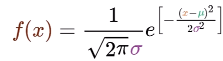
1、高斯正态分布函数（正态分布）

如下图所示，为正态分布的概率密度曲线，俗称 "钟形曲线" ：

其中， f(x) 为概率密度（无实际含义），x 为随机变量。e 和 π 为常量（就是那两个值）。μ 为随机变量的平均值，名为期望，是钟形曲线的 "对称轴"。σ 为为随机变量的标准差，名为方差。μ 和 σ 决定了钟形曲线的位置和形状，因此只需要确定μ 和 σ 就可以确定正态分布函数的概率密度函数。所以，正态分布函数也常表示为 $N(\mu, \sigma^2)$ ，N表示 Normal（正态）。概率密度曲线和x轴之间合围的面积区域表示随机变量区间内发生的概率。

2. 高斯噪声

期望 μ 为0，方差 σ 为1的正态分布，为标准正态分布 $N(0,1)$ 。从一个标准正态分布中 "随机抽取" 样本，生成一组符合该分布的随机变量值，这样一组变量就叫做 "标准正态分布随机变量" ，在用于制造向数据中添加的噪声时，也叫做 "高斯噪声"。这样一组随机变量值，即是 "高斯噪声值"。

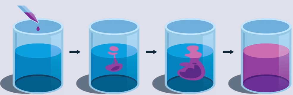
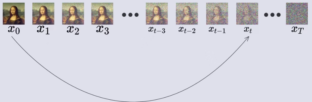
3. 扩散现象和扩散模型

当一滴墨水滴入水中时，随着时间的推移，由于分子之间的碰撞和热运动，墨水分子开始向周围扩散。

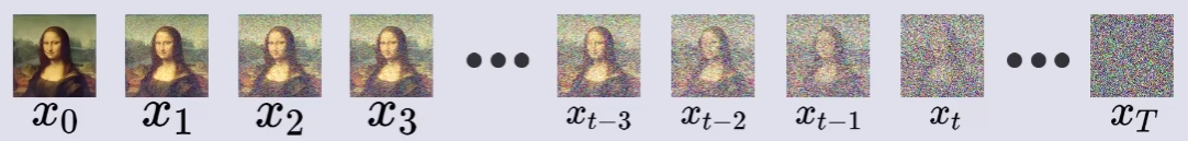
扩散模型受到这种现象的启发，通过逐步向图片中添加高斯噪声来模拟这种现象（最终图像会变成一张符合 $N(0,1)$ 的纯噪声），并通过逆向过程逐步从噪声中生成图像（通过模型学习去噪过程）。

这样做的好处在于，一个训练好的完备的模型可以通过逆向过程从任意的符合 $N(0,1)$ 的纯噪声中生成图像，使得生成样本具有较高的质量和多样性。

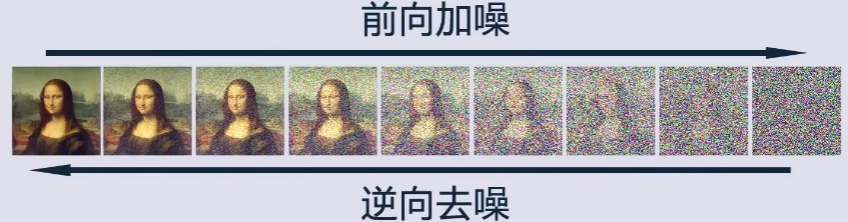
4. 扩散模型的前向过程（加噪过程)

那么，扩散模型 的具体加噪过程，应该怎么实现呢？

首先，为加噪图片创造出一张等大小的高斯噪声图片。

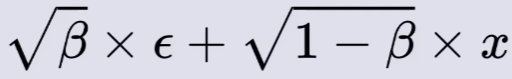
通过以下公式实现高斯噪声图片与输入图像的混合：

其中，x 为输入图像，ϵ 为等大小的高斯噪声图片，β 为产生 x 和 ϵ 系数的参数值（β 仅仅只是一个参数值，用于调和高斯噪声和输入图像的混合比例）。

如上图所示，加噪的过程是一个连续的，具有稳定时间步数的过程，且每一步加噪结果仅依赖于上一步的样本，这便是一个马尔可夫链。（简述马尔可夫链【通俗易懂】）

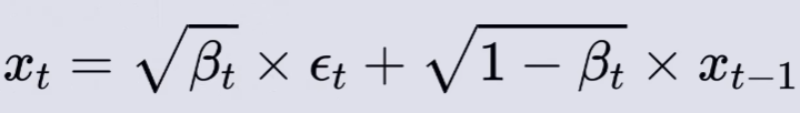
以上图为例，可以得到一个🌟新的公式，如下所示：

其中，加噪所使用的噪声 $\epsilon _t$ 是基于标准正态分布 $\epsilon_t\sim N(0,1)$ 随机采样得来的。 $\beta_t \in (1,0)$ 并且随着步数逐渐增大，因为扩散速度是越来越快的。

5. 高斯函数叠加和重参数化技巧（扩散模型的前向过程的继续推导）

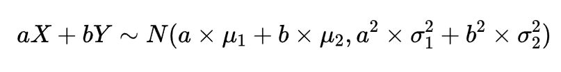
在得出上述公式之后，我们仅需要知道高斯函数叠加公式（ $\epsilon _t$ 符合标准高斯分布 $\epsilon_t\sim N(0,1)$ ），就能知道最终加噪结果。

简单来讲，🌟给定两个高斯分布 $X\sim N(\mu_{1} , \sigma_{1} ^{2})$ 和 $Y\sim N(\mu_{2} , \sigma_{2} ^{2})$ 进行叠加，则它们叠加后的分布 $aX+bY$ 满足：

那么继续 扩散模型的前向过程 的推导，首先，为了方便计算，令 β =1 - α ：

代入 $X_{t-1}$ ：

已知 $\epsilon_t\sim N(0,1)$ ，根据高斯函数叠加公式：

🌟重参数化，得

（没错，这便是重参数化，在数学中仅仅只是一个将高斯函数简式表示重整为等式的方法。但是在梯度传播过程中，由于 $\epsilon _t$ 是随机采样得来的，那么与之对应的加噪样本 $X_{t}$ 也是随机生成的，这样的样本在 前向过程 的每个阶段都存在，导致梯度无法传播。通过重参数化，随机采样的噪声 $\epsilon _t$ 被压缩到只有一个 $\epsilon$ ，这样一个随机噪声生成之后不会再变，与之对应的加噪样本也不会再变，对梯度传播不会产生影响）

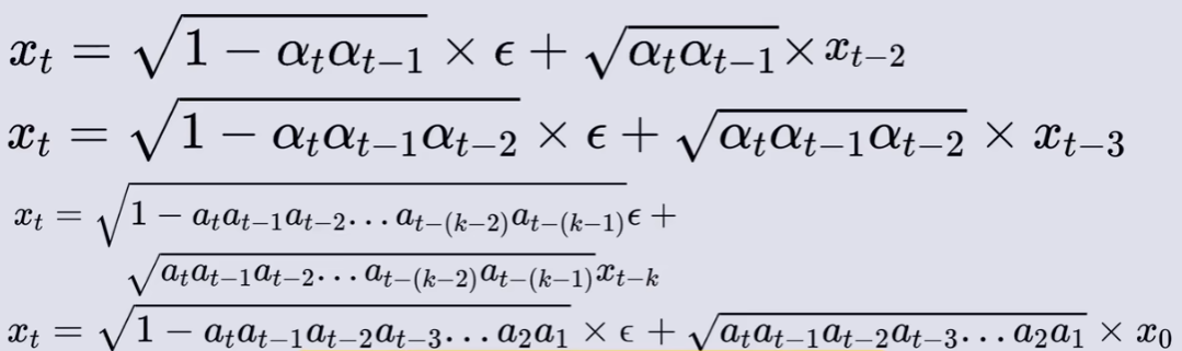
重复上述过程可得：

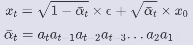
其中a_t a_{t-1} a_{t-2}...a1很长，为了方便表达，用 $\bar{\alpha }_t$ 代替：

最后，我们得到了最终加噪结果。

不难看出，最终加噪结果 xt 是由 x0 直接得出而来的（重参数化）。这是"迫于"随机采样导致梯度无法传播而做的选择。（也不好说，这种做法，说不定效果更优呢）。

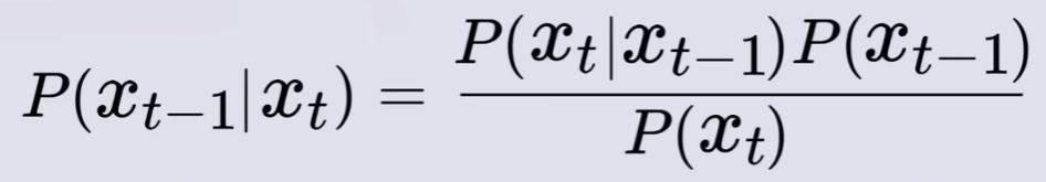
6. 贝叶斯公式和反向过程

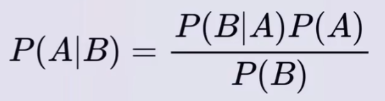
贝叶斯公式，如下：

其中，A、B 表示随机事件A和随机事件B。P(A) 和 P(B) 表示事件A和事件B发生的概率。P(B|A) 表示A事件发生的情况下B事件发生的概率。P(A|B) 表示B事件发生的情况下A事件发生的概率。贝叶斯公式强调 “已知结果找原因”。P(A) 是先验概率，P(A|B) 是后验概率。

（🌟同样，贝叶斯是可以求取后验概率分布，因为某一类的概率和某一类的概率分布只是定义上不同，本质上都是概率对不同事件的划分）

反向过程推导：

🌟由于在前向过程中从前一时刻向后一时刻加入的是根据正态分布随机采样的噪声，所以从 $X_t$ 到 $X_{t-1}$ 也应该是一个随机过程，我们无法简单地预测 $X_t$ 到 $X_{t-1}$ 的样本和具体的噪声值，但是我们可以通过贝叶斯公式大致地推测出给定 $X_t$ 条件下 $X_{t-1}$ 噪声的概率分布。（注意，这里已知的 $X_t$ 条件，是指最终加噪结果 $X_t$ 的噪声的概率分布 $\epsilon \sim N(0,1 - \bar{\alpha} )$ ）

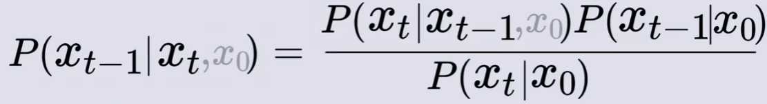
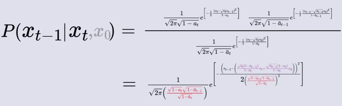
由贝叶斯公式得：

表示为由x0原图 “得到” 作为条件，得：

其中， $P(x_{t-1}| x_t,x_0)$ 表示在给定Xt的情况下得到X_{t-1}的概率（反向过程中）， $P(x_t| x_{t-1},x_0)$ 表示在给定X_{t-1}的情况下得到Xt的概率（正向过程中）， $P(x_t|x_0)$ 从X0原图得到Xt的概率， $P(x_{t-1}| x_0)$ 从X0原图得到X_{t-1}的概率。（这里概率都指的得到对应概率分布的概率）。

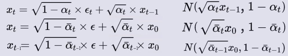
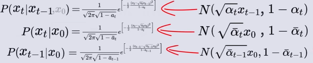
由正向过程给出的推断式可得， $P(x_t| x_{t-1},x_0)$ ， $P(x_t|x_0)$ ， $P(x_{t-1}| x_0)$ 对应正态分布表达式分别如下所示：

代入高斯正态分布函数可得：

代回贝叶斯公式，得

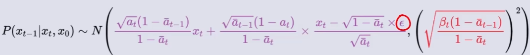
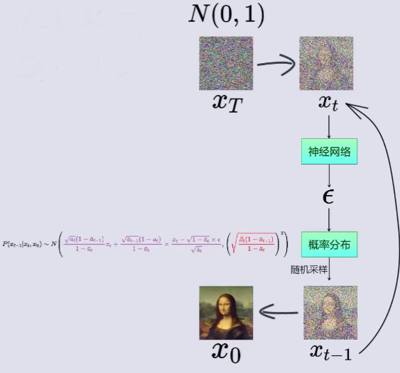
这样，我们就可以推测出给定 $X_t$ 条件下 $X_{t-1}$ （包含噪声）的概率分布。其中 $X_t$ 是正向过程中最终得加噪结果， $\bar{\alpha }$ 和 $\beta$ 是无实际含义的参数， $\epsilon$ 是从一个标准正态分布中 "随机抽取" 的噪声样本。🌟而 $\epsilon$ 是图像去噪的关键，只有找到与正向过程一致或接近的随机采样噪声值（噪声的概率分布已推测出）才能顺利还原图像，🌟 $\epsilon$ 由神经网络模型进行学习输出（只学习这个值）。

不断重复上述过程，最终得到原图像 X0 的概率分布。如下图所示（该图只是一个大概过程，并不符合事实）：

在推测出每个阶段的噪声的概率分布后，神经网络模型不断地学习优化 $\epsilon$ 。

一、摘要

研究动机：本文提出使用扩散概率模型得到高质量图像的合成结果，这是一类受非平衡热力学考虑启发的潜在变量模型。

主要工作：本文的最佳结果是通过在 加权变分界 上进行训练获得的，该变分界是根据 扩散概率模型 和与Langevin动力学匹配的 去噪分数 之间的新联系设计的，并且本文的模型自然地允许 渐进有损解压缩方案 ，可以解释为自回归解码的推广。（目标函数：变分推断，KL散度 + 模型：扩散概率模型和去噪分数 + 采样方式：渐进式编码和渐进式解码）

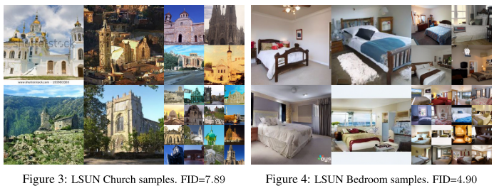
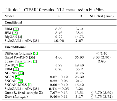
实验结果：在CIFAR10数据集上，本文方法获得了9.46的Inception分数和3.17的最新FID分数。在256x256 LSUN上，本文方法获得了类似ProgressiveGAN的样品质量。

二、引言

相关工作概述（生成对抗网络(gan)、自回归模型、流和变分自编码器(VAEs) ） —> 扩散概率模型概述（ “扩散模型”是一个参数化的马尔可夫链，使用变分推理进行训练 + 正向过程概述 + 反向过程概述）—> 模型效果概述+ 扩散模型某些参数化设计 +采样方式概述

三、主要方法

扩散模型是形式为 $p_\theta (x_0):= \int p_\theta (x_{0:T}) dx_{1:T}$ 的隐变量模型，其中x1，…，xT是与数据x0 ~ q(x0)相同维数的潜变量。

反向过程定义（逆扩散过程）：联合分布 $p_\theta (x_{0:T})$ 被称为反向过程，它被定义为一个马尔可夫链，其中学习高斯转移从 $p(x_T) = N(x_T;0, I)$ 开始：

$p_\theta$ 表示噪声的概率分布。这里左半部分 $p_\theta (x_{0:T})$ 是的简化，是 x0,…,xT 的联合密度函数，表示给定xT ,…, x1条件下x0 噪声的概率分布（这是一个逆向推断的过程，推理到x0时，xT ,…, x1的噪声的概率分布已全部给定）。右半部分 $p_\theta (x_{t-1}|x_t):= N(x_{t-1};\mu _\theta (x_t, t),\Sigma _\theta(x_T,T))$ 表示给定 $X_t$ 条件下 $X_{t-1}$ 噪声的概率分布。

前向过程定义（扩散过程）：扩散模型与其他类型的隐变量模型的区别在于，近似后验 $q(x_{1:T}|x_0)$ ，称为前向过程或扩散过程，固定在一个马尔可夫链中，逐渐向数据中添加高斯噪声根据方差 β1, . . ., βT：

β 表示原图与噪声的混合比例（详情看论文铺垫部分）。

优化函数：在训练过程中使用负对数似然的变分界限进行优化：

对𝑝𝜃(𝑥0) 的最大似然估计进行优化。

任意时刻的 xt 可以由 x0 和 β 表示：正向过程的一个显著特性是，它允许在任意时间步长 t 上以闭合形式对 xt 进行采样：使用符号 $\alpha _t:= 1-\beta_t$ 和 $\bar{\alpha }_t:=\sum^t _{s=1} \alpha _s$ ，有

对应论文铺垫前向过程中最后一部分。由重参数化实现。

代码实现：

class GaussianDiffusion:
    """
    Utilities for training and sampling diffusion models.
    Ported directly from here, and then adapted over time to further experimentation.
    https://github.com/hojonathanho/diffusion/blob/1e0dceb3b3495bbe19116a5e1b3596cd0706c543/diffusion_tf/diffusion_utils_2.py#L42
    :param betas: a 1-D numpy array of betas for each diffusion timestep,
                  starting at T and going to 1.
    :param model_mean_type: a ModelMeanType determining what the model outputs.
    :param model_var_type: a ModelVarType determining how variance is output.
    :param loss_type: a LossType determining the loss function to use.
    :param rescale_timesteps: if True, pass floating point timesteps into the
                              model so that they are always scaled like in the
                              original paper (0 to 1000).
    """

    def __init__(
        self,
        *,
        betas,
        model_mean_type,
        model_var_type,
        loss_type,
        dpm_solver,
        rescale_timesteps=False,
    ):
        self.model_mean_type = model_mean_type
        self.model_var_type = model_var_type
        self.loss_type = loss_type
        self.rescale_timesteps = rescale_timesteps
        self.dpm_solver = dpm_solver

        # Use float64 for accuracy.
        betas = np.array(betas, dtype=np.float64)
        self.betas = betas
        assert len(betas.shape) == 1, "betas must be 1-D"
        assert (betas > 0).all() and (betas <= 1).all()

        self.num_timesteps = int(betas.shape[0])

        alphas = 1.0 - betas
        self.alphas_cumprod = np.cumprod(alphas, axis=0)
        self.alphas_cumprod_prev = np.append(1.0, self.alphas_cumprod[:-1])
        self.alphas_cumprod_next = np.append(self.alphas_cumprod[1:], 0.0)
        assert self.alphas_cumprod_prev.shape == (self.num_timesteps,)

        # calculations for diffusion q(x_t | x_{t-1}) and others
        self.sqrt_alphas_cumprod = np.sqrt(self.alphas_cumprod)
        self.sqrt_one_minus_alphas_cumprod = np.sqrt(1.0 - self.alphas_cumprod)
        self.log_one_minus_alphas_cumprod = np.log(1.0 - self.alphas_cumprod)
        self.sqrt_recip_alphas_cumprod = np.sqrt(1.0 / self.alphas_cumprod)
        self.sqrt_recipm1_alphas_cumprod = np.sqrt(1.0 / self.alphas_cumprod - 1)

        # calculations for posterior q(x_{t-1} | x_t, x_0)
        self.posterior_variance = (
            betas * (1.0 - self.alphas_cumprod_prev) / (1.0 - self.alphas_cumprod)
        )
        # log calculation clipped because the posterior variance is 0 at the
        # beginning of the diffusion chain.
        self.posterior_log_variance_clipped = np.log(
            np.append(self.posterior_variance[1], self.posterior_variance[1:])
        )
        self.posterior_mean_coef1 = (
            betas * np.sqrt(self.alphas_cumprod_prev) / (1.0 - self.alphas_cumprod)
        )
        self.posterior_mean_coef2 = (
            (1.0 - self.alphas_cumprod_prev)
            * np.sqrt(alphas)
            / (1.0 - self.alphas_cumprod)
        )

    def q_mean_variance(self, x_start, t):
        """
        Get the distribution q(x_t | x_0).
        :param x_start: the [N x C x ...] tensor of noiseless inputs.
        :param t: the number of diffusion steps (minus 1). Here, 0 means one step.
        :return: A tuple (mean, variance, log_variance), all of x_start's shape.
        """
        mean = (
            _extract_into_tensor(self.sqrt_alphas_cumprod, t, x_start.shape) * x_start
        )
        variance = _extract_into_tensor(1.0 - self.alphas_cumprod, t, x_start.shape)
        log_variance = _extract_into_tensor(
            self.log_one_minus_alphas_cumprod, t, x_start.shape
        )
        return mean, variance, log_variance

    def q_sample(self, x_start, t, noise=None):
        """
        Diffuse the data for a given number of diffusion steps.
        In other words, sample from q(x_t | x_0).
        :param x_start: the initial data batch.
        :param t: the number of diffusion steps (minus 1). Here, 0 means one step.
        :param noise: if specified, the split-out normal noise.
        :return: A noisy version of x_start.
        """
        if noise is None:
            noise = th.randn_like(x_start)
        assert noise.shape == x_start.shape
        return (
                _extract_into_tensor(self.sqrt_alphas_cumprod, t, x_start.shape) * x_start
                + _extract_into_tensor(self.sqrt_one_minus_alphas_cumprod, t, x_start.shape)
                * noise
        )

    def q_posterior_mean_variance(self, x_start, x_t, t):
        """
        Compute the mean and variance of the diffusion posterior:
            q(x_{t-1} | x_t, x_0)
        """
        assert x_start.shape == x_t.shape
        posterior_mean = (
            _extract_into_tensor(self.posterior_mean_coef1, t, x_t.shape) * x_start
            + _extract_into_tensor(self.posterior_mean_coef2, t, x_t.shape) * x_t
        )
        posterior_variance = _extract_into_tensor(self.posterior_variance, t, x_t.shape)
        posterior_log_variance_clipped = _extract_into_tensor(
            self.posterior_log_variance_clipped, t, x_t.shape
        )
        assert (
            posterior_mean.shape[0]
            == posterior_variance.shape[0]
            == posterior_log_variance_clipped.shape[0]
            == x_start.shape[0]
        )
        return posterior_mean, posterior_variance, posterior_log_variance_clipped


    def p_mean_variance(
        self, model, x, t, clip_denoised=True, denoised_fn=None, model_kwargs=None
    ):
        """
        Apply the model to get p(x_{t-1} | x_t), as well as a prediction of
        the initial x, x_0.
        :param model: the model, which takes a signal and a batch of timesteps
                      as input.
        :param x: the [N x C x ...] tensor at time t.
        :param t: a 1-D Tensor of timesteps.
        :param clip_denoised: if True, clip the denoised signal into [-1, 1].
        :param denoised_fn: if not None, a function which applies to the
            x_start prediction before it is used to sample. Applies before
            clip_denoised.
        :param model_kwargs: if not None, a dict of extra keyword arguments to
            pass to the model. This can be used for conditioning.
        :return: a dict with the following keys:
                 - 'mean': the model mean output.
                 - 'variance': the model variance output.
                 - 'log_variance': the log of 'variance'.
                 - 'pred_xstart': the prediction for x_0.
        """
        if model_kwargs is None:
            model_kwargs = {}
        B, C = x.shape[:2]
        C=1
        cal = 0
        assert t.shape == (B,)
        model_output = model(x, self._scale_timesteps(t), **model_kwargs)
        if isinstance(model_output, tuple):
            model_output, cal = model_output
        x=x[:,-1:,...]  #loss is only calculated on the last channel, not on the input brain MR image
        if self.model_var_type in [ModelVarType.LEARNED, ModelVarType.LEARNED_RANGE]:
            assert model_output.shape == (B, C * 2, *x.shape[2:])
            model_output, model_var_values = th.split(model_output, C, dim=1)
            if self.model_var_type == ModelVarType.LEARNED:
                model_log_variance = model_var_values
                model_variance = th.exp(model_log_variance)
            else:
                min_log = _extract_into_tensor(
                    self.posterior_log_variance_clipped, t, x.shape
                )
                max_log = _extract_into_tensor(np.log(self.betas), t, x.shape)
                # The model_var_values is [-1, 1] for [min_var, max_var].
                frac = (model_var_values + 1) / 2
                model_log_variance = frac * max_log + (1 - frac) * min_log
                model_variance = th.exp(model_log_variance)
        else:
            model_variance, model_log_variance = {
                # for fixedlarge, we set the initial (log-)variance like so
                # to get a better decoder log likelihood.
                ModelVarType.FIXED_LARGE: (
                    np.append(self.posterior_variance[1], self.betas[1:]),
                    np.log(np.append(self.posterior_variance[1], self.betas[1:])),
                ),
                ModelVarType.FIXED_SMALL: (
                    self.posterior_variance,
                    self.posterior_log_variance_clipped,
                ),
            }[self.model_var_type]
            model_variance = _extract_into_tensor(model_variance, t, x.shape)
            model_log_variance = _extract_into_tensor(model_log_variance, t, x.shape)

        def process_xstart(x):
            if denoised_fn is not None:
                x = denoised_fn(x)
            if clip_denoised:
                return x.clamp(-1, 1)
            return x

        if self.model_mean_type == ModelMeanType.PREVIOUS_X:
            pred_xstart = process_xstart(
                self._predict_xstart_from_xprev(x_t=x, t=t, xprev=model_output)
            )
            model_mean = model_output
        elif self.model_mean_type in [ModelMeanType.START_X, ModelMeanType.EPSILON]:
            if self.model_mean_type == ModelMeanType.START_X:
                pred_xstart = process_xstart(model_output)
            else:
                pred_xstart = process_xstart(
                    self._predict_xstart_from_eps(x_t=x, t=t, eps=model_output)
                )
            model_mean, _, _ = self.q_posterior_mean_variance(
                x_start=pred_xstart, x_t=x, t=t
            )
        else:
            raise NotImplementedError(self.model_mean_type)

        assert (
            model_mean.shape == model_log_variance.shape == pred_xstart.shape == x.shape
        )
        return {
            "mean": model_mean,
            "variance": model_variance,
            "log_variance": model_log_variance,
            "pred_xstart": pred_xstart,
            'cal': cal,
        }

四、实验

实验细节：为所有实验设置T = 1000，以便采样期间所需的神经网络评估数量与之前的工作相匹配。将正向过程方差设置为常数，从 $\beta_1 = 10^{-4}$ 到 $\beta_T = 10^{-4}$ 线性增加。在实验中 $L_T = D_{KL}(q(x_T|x_0) || N(0, I)) \approx 10^5$ 。为了表示反向过程，使用类似于未掩码的PixelCNN+的U-Net骨干，并始终进行group normalization。参数是跨时间共享的，使用Transformer正弦位置嵌入对网络进行指定。在16 × 16特征图分辨率上使用自注意力。

4.1 图片生成质量

在 CIFAR10 数据集上，在训练集上，无条件模型 FID 分数达到 3.17；在测试集上 FID 分数为5.24，图片质量超过其他模型。

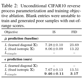
4.2 损失函数比较

简化损失函数的影响，结果如下表：

五、结论

1. 主要工作：本文发现了扩散模型和变分推断之间的联系，用于训练马尔可夫链、去噪分数匹配、自回归模型和渐进损耗压缩。

2. 实验效果：在 CIFAR10 数据集上，在训练集上，无条件模型 FID 分数达到 3.17。在测试集上 FID 分数为5.24，图片质量超过其他模型。

向岸看

关注

32
点赞
踩
35

收藏

觉得还不错? 一键收藏
打赏
0
评论
Denoising Diffusion Probabilistic Models 全过程概述 + 论文总结

DDPM全过程概述，扩散模型 = 高斯正态分布函数 + 马尔可夫链 + 高斯函数叠加 + 重参数化 + 贝叶斯公式。
复制链接

扫一扫