深度学习模型部署(番外4)模型量化方案及实战

量化方案

根据量化的时机可以分为训练时量化QAT和训练后量化PTQ。二者的工作流程图如下：

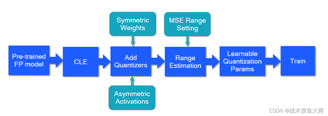
QAT量化流程图

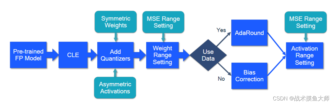
PTQ量化流程图

其中的CLE为层间放缩平衡Cross-Layer Equalization，在使用per_tensor粒度进行量化时，同一个tensor中可能数据不平衡情况很严重，尤其是在深度可分离卷积中，非常影响量化性能，所以为了解决这个问题提出的，大致可以理解为对于前后两层，前面一层的参数放大s倍，后面一层的参数缩小s倍，那么最后的输出结果不会有太大变化。关于CLE后面在量化性能调优的blog里面讲

PTQ

其中PTQ又分为PTDQ和PTSQ两种方案，二者的主要区别是对于activation的处理不同。具体区别如下：

PTDQ

Post Training Dynamic Quantization,训练后动态量化，也就是在模型训练收敛后进行量化，weight进行量化，而activation则是在推理过程中进行动态计算scale和offset，进行动态量化。
这种方案是最简单的量化方案，主要用于模型参数加载较为费时的模型，如LSTM和transformer。
具体的参数类型如下：

# original model
# all tensors and computations are in floating point
previous_layer_fp32 -- linear_fp32 -- activation_fp32 -- next_layer_fp32
                 /
linear_weight_fp32

# dynamically quantized model
# 只有weight变成了int8，activation还是fp32
previous_layer_fp32 -- linear_int8_w_fp32_inp -- activation_fp32 -- next_layer_fp32
                     /
   linear_weight_int8

pytorch demo代码如下：

import torch

# define a floating point model
class M(torch.nn.Module):
    def __init__(self):
        super().__init__()
        self.fc = torch.nn.Linear(4, 4)

    def forward(self, x):
        x = self.fc(x)
        return x

model_fp32 = M()
# create a quantized model instance
model_int8 = torch.ao.quantization.quantize_dynamic(
    model_fp32,  # the original model
    {torch.nn.Linear},  # 自己选择要进行量化的层
    dtype=torch.qint8)  # 量化后参数的存储类型

# run the model
input_fp32 = torch.randn(4, 4, 4, 4)
res = model_int8(input_fp32)

PTSQ

Post Training Static Quantization，训练后静态量化。
与PTDQ的不同在于，PTSQ是把weight和activation的量化都提前做好，等到推理时不需要涉及到任何计算scale和offset的工作。对于activation的量化，PTSQ会尽量把它融合到前一层中，跟一层的layer一块儿量化。
这种方案适合读取参数和计算都比较耗时的模型，读取参数时间和计算时间都减少了。但是需要采用典型的数据进行校准，用于提前计算activation的scale和offset。
pytorch中PTSQ的方案需要自己定义量化器和解量化器，并且自己定义哪里开始量化，哪几层进行融合。

# original model
previous_layer_fp32 -- linear_fp32 -- activation_fp32 -- next_layer_fp32
                    /
    linear_weight_fp32

# statically quantized model
# 将linear和activation融合到了一块儿
previous_layer_int8 -- linear_with_activation_int8 -- next_layer_int8
                    /
  linear_weight_int8

pytorch代码如下：

import torch

# define a floating point model where some layers could be statically quantized
class M(torch.nn.Module):
    def __init__(self):
        super().__init__()
        self.quant = torch.ao.quantization.QuantStub() # 量化器
        self.conv = torch.nn.Conv2d(1, 1, 1)
        self.relu = torch.nn.ReLU()
        self.dequant = torch.ao.quantization.DeQuantStub() # 解量化器

    def forward(self, x):
        x = self.quant(x) # 将x量化，由FP32变成int8
        x = self.conv(x)
        x = self.relu(x)
        x = self.dequant(x) # 解量化，由int8变回FP32
        return x

# create a model instance
model_fp32 = M()

model_fp32.eval()

model_fp32.qconfig = torch.ao.quantization.get_default_qconfig('x86')


# Common fusions include `conv + relu` and `conv + batchnorm + relu`
model_fp32_fused = torch.ao.quantization.fuse_modules(model_fp32, [['conv', 'relu']])
model_fp32_prepared = torch.ao.quantization.prepare(model_fp32_fused)

input_fp32 = torch.randn(4, 1, 4, 4) //典型数据
model_fp32_prepared(input_fp32) //校准，计算scale和offset

model_int8 = torch.ao.quantization.convert(model_fp32_prepared) //模型转化

res = model_int8(input_fp32) //推理

QAT

边量化边训练，训练过程还是浮点数运算，不过会进行量化模拟，模拟量化以查看效果，本来训练是使loss最小，QAT情况下的训练是：使量化模拟后的模型loss最小。

关于量化模拟在之前提到过，详见：tensor量化
加入量化器后出现的一个问题就是：反向传播的时候，量化模拟器怎么求导？量化模拟器求导的结果要么是0要么就是不存在，所以这里引入直通估计，也就是假设四舍五入函数$round(x)$的导数为1，也就是不影响求导，最终的反向传播效果如下：

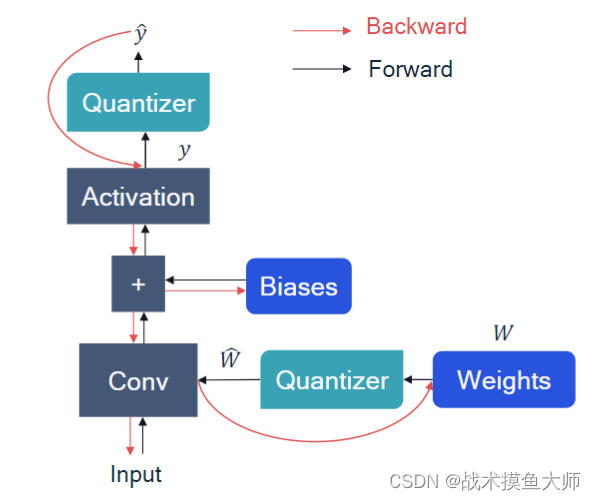
量化前后数据流图：

# original model
previous_layer_fp32 -- linear_fp32 -- activation_fp32 -- next_layer_fp32
                      /
    linear_weight_fp32

# 量化模拟，在其中加入了很多量化器，为了模拟量化产生的精度损失，数据依旧使fp32类型
previous_layer_fp32 -- fq -- linear_fp32 -- activation_fp32 -- fq -- next_layer_fp32
                           /
   linear_weight_fp32 -- fq

# 真实量化过的模型，全部都是int8
previous_layer_int8 -- linear_with_activation_int8 -- next_layer_int8
                     /
   linear_weight_int8

demo代码：

import torch

# define a floating point model where some layers could benefit from QAT
class M(torch.nn.Module):
    def __init__(self):
        super().__init__()
        self.quant = torch.ao.quantization.QuantStub() //量化器
        self.conv = torch.nn.Conv2d(1, 1, 1)
        self.bn = torch.nn.BatchNorm2d(1)
        self.relu = torch.nn.ReLU()
        self.dequant = torch.ao.quantization.DeQuantStub() //解量化器

    def forward(self, x):
        x = self.quant(x)
        x = self.conv(x)
        x = self.bn(x)
        x = self.relu(x)
        x = self.dequant(x)
        return x

def training_loop(model):
	pass

# create a model instance
model_fp32 = M()
model_fp32.eval()

model_fp32.qconfig = torch.ao.quantization.get_default_qat_qconfig('x86')

# 算子融合，将多个算子融合为一个
model_fp32_fused = torch.ao.quantization.fuse_modules(model_fp32,
    [['conv', 'bn', 'relu']])

# 准备量化
model_fp32_prepared = torch.ao.quantization.prepare_qat(model_fp32_fused.train())

# 训练
training_loop(model_fp32_prepared)

model_fp32_prepared.eval()
model_int8 = torch.ao.quantization.convert(model_fp32_prepared)

res = model_int8(input_fp32)

pytorch对于量化的实现

量化算法支持

回归到最底层的tensor量化，有两种量化粒度：per_tensor和per_channel，两种量化方法：对称量化，非对称量化。一共2*2=4种选择，所以pytorch也提供了4种方法：

import torch
torch.per_tensor_affine # 非对称
torch.per_tensor_symmetric # 对称
torch.per_channel_affine
torch.per_channel_symmetric

量化不仅仅需要进行模型融合，加入量化算法支持，还需要对tensor进行修改，原本的tensor只需要存储数据，现在对于量化过的INT8 tensor，还需要存储scale和offset。所以pytorch针对量化后的tensor提供了新的类型：

import torch
torch.quint8
torch.qint8
torch.qint32
torch.float16

关于config，类型转化等，详见官方文档：官方文档

如果觉得有帮助，请点赞收藏+关注，thanks