Silvaco学习笔记（十四）——获取器件特性（毕设相关）

一、获取器件特性（唐龙谷老师书籍学习）

在仿真开始时电极都是零偏的，之后才会按照设置的方式将电流或电压步进式地加上 去。步进的步长是需要考虑的，步长太大容易不收敛（由于计算方法中的初始猜测策略）。

电压和电流的施加使用 solve 状态， log 和 save 是将计算得到结果分别保存为日志文件和结 构文件。 Log 语句需要在 solve 之前，这样 solve 的数据才能得到保存。

示例：

log outfile=test.log 
solve vgate=0.1 
save outfile=gate_0.1.str

1.1 直流特性

例1：所有电极电压加到0V

solve init

经过 solve 之后保存的结构文件中将包含有电学信息（电势，电流密度，电极的电流电压等）。直接从某一电压开始计算，则上面的语句 solve init 将 自动加入 。

例2：基极电压加到0.1V

solve vbase=0.1

例3：将之前计算得到的结果作为计算的初始近似

solve previous

例4：结束写日志

log off

例5：基极电压经过一系列步骤加到 2.0V，可以得到 BE 结的 I-V 特性

go atlas 
init infile=SBD.str 
# 
model conmob fldmob srh auger bgn 
contact name=anode workf=4.97
solve init
log outfile=Schottky_Diode_IV.log
solve vanode=0.01 
solve vanode=0.05
solve vanode=0.1 
solve vanode=0.15 
…
solve vanode=2.0 
tonyplot Schottky_Diode_IV.log

这个是“分立”的

例6：栅电压按一定步长进行扫描，可得转移特性，从保存的日志文件中可提取出跨 导随栅压的特性曲线。如果 vfinal 不是整数个步长后的值，则会自动调整。

go atlas
init infile=structure.str 
models cvt srh print
# 
contact name=gate n.poly
interface qf=3e10
# 
method newton
solve init
solve vdrain=0.1
log outf=Vt_test.log master
solve vgate=0.1 vstep=0.1 vfinal=3.0 name=gate
tonyplot Vt_test.log 
quit

这个是“集中”的

例7：Gummel Plot 特性仿真

go atlas 
init infile=bjt.str 
models conmob fldmob consrh auger print 
solve init
solve vcollector=0.1 vstep=0.1 vfinal=2 name=collector
log outf=Gummel_Plot.log
solve vbase=0.025 vstep=0.025 vfinal=1 name=base
log off
tonyplot Gummel_Plot.log
quit

例8：电极短接来得到GP特性

contact name=base common=collector
log outf=gp.log
solve vbase=0.0 vstep=0.1 vfinal=2 name=base

BJT 的 CE 结击穿特性的仿真须将基极开路，开路接触在介绍接触时也提到了，实现的方法是将基极定义成电流控制电极，再将电流设置成很小的接近于零的值。

例9：击穿特性仿真

go atlas
init infile=bjt.str 
models bipolar print
impact selb
method trap climit=1e-4 maxtrap=10
#
solve vbase=0.2
#
contact name=base current
solve ibase=3.e-15
#
log outfile=breakdown.log master
#
solve vcollector=0.2 vstep=0.2 vfinal=5 name=collector
solve vstep=0.5 vfinal=10 name=collector compl=5.e-10 e.comp=3 
tonyplot breakdown.log

通常会分段扫描电压，开始阶段的步长小一点以利于计算收敛，然后适当增加步长。此例就是分段扫描电压的一个例子。

在仿真击穿特性时必须使用碰撞离化模型。上例 solve 中参数 comp 为限流致 5e-10A， 参数 e.comp 将限流的电极数设置为 3 。

电流控制型器件（ BJT ， HBT ）的输出特性仿真，是一个 Ib 一条曲线的。读者如果够细 心的话则会发现上面仿真击穿特性的语句实际上就是输出特性曲线中 Ib=0 （ 3e-15≈ 0）的那 一条。按照这个思路，在解得的每一个 Ib 值后保存一下结构文件（结构文件中里面要有当 时完整的电学信息），再在扫描集电极电压时导入相应的结构文件即可得到输出特性。

例10：电流控制型器件的输出特性仿真。

…
solve init
solve vbase=0.05 vstep=0.05 vfinal=0.8 name=base
contact name=base current
#
solve ibase=1.e-6
save outf=bjt_ib_1.str master
solve ibase=2.e-6 
save outf=bjt_ib_2.str master
solve ibase=3.e-6 
save outf=bjt_ib_3.str master
solve ibase=4.e-6
save outf=bjt_ib_4.str master 
solve ibase=5.e-6
save outf=bjt_ib_5.str master
#
load inf=bjt_ib_1.str master
log outf=bjt_ib_1.log
solve vcollector=0.0 vstep=0.25 vfinal=5.0 name=collector
#
load inf=bjt_ib_2.str master
log outf=bjt_ib_2.log
solve vcollector=0.0 vstep=0.25 vfinal=5.0 name=collector
# 
load inf=bjt_ib_3.str master
log outf=bjt_ib_3.log 
solve vcollector=0.0 vstep=0.25 vfinal=5.0 name=collector
# 
load inf=bjt_ib_4.str master
log outf=bjt_ib_4.log 
solve vcollector=0.0 vstep=0.25 vfinal=5.0 name=collector
…
tonyplot –overlay bjt_ib_*.log
quit

语句中 bjt_ib_*.str 为一定基极电流下保存的结构文件

bjt_ib_*.log 为对应的输出特性曲线。

Save 状态中的 master 参数将计算得到的电学特性保存在结构文件中

电压控制型器件（MOS，MESFET，HEMT）的输出特性仿真和电流控制型器件的方法类似。有时栅电压跨度大，为了收敛需要将 method 的参数 maxtrap 设置大一些。

例11： 电压控制型器件的输出特性仿真

…
solve init 
solve vgate=1 outf=solve_tmp1
solve vgate=2 outf=solve_tmp2
#
load infile=solve_tmp1
log outf=mos_ids_1.log 
solve name=drain vdrain=0 vstep=0.3 vfinal=3.3
#
load infile=solve_tmp2
log outf=mos_ids_2.log 
solve name=drain vdrain=0 vstep=0.3 vfinal=3.3 
…
tonyplot –overlay mos_ids_*.log

这个_*的写法真方便呀，回头试试

1.2 交流小信号特性

交流仿真的语法和直流仿真的语法很相似，只是添加了频率相关的参数。有两种交流仿

真类型，一是频率不变只变直流偏置，一是变频率直流偏置不变。

例1： 交流仿真，频率不变，变直流偏置（能得到特定频率下的 CV 特性）。

solve vgate=-5 vstep=0.1 vfinal=5.0 name=gate ac freq=1e6

例2：交流仿真，变交流频率（能得到两端口的电容随频率变化的特性）。频率从 1GHz 增加到 11GHz，以 1GHz 为步长。

solve vbase=0.7 ac freq=1e9 fstep=1e9 nfstep=10

例3：交流仿真，在初始频率的基础上按倍数增加，从 1MHz 开始，频率每一次增加为原来的两倍，总共增加 10 次，这样最后为 2^10*1MHz=1.024GHz。

solve vbase=0.7 ac freq=1e6 fstep=2 mult.f nfstep=10

例4：直流偏置和交流频率一起改变，这会在每一个直流偏置点都对频率进行扫描。

solve vgate=0 vstep=0.05 vfinal=1 name=gate ac freq=1e6 fstep=2 mult.f nfsteps=10

1.3 瞬态特性

瞬态仿真用于时间相关的测试或响应。瞬态仿真可以由逐段线性方式，指数函数方式和正弦函数方式获得。

例1： 在 ramptime 时间内栅压加到 1.0V ，然后保持直到 tstop

solve vgate=1.0 ramptime=1e-9 tstep=0.1e-9 tstop=1e-8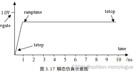

 1.4 高级特性

1. curvetrace

Curvetrace 可以设置复杂的扫描方式，自动得到 I-V 特性。 curvetrace 和 solve 联合使用

可用于击穿电压仿真、 CMOS 栓锁仿真和二次击穿仿真。

例1： curcetrace 定义扫描方式。

curvetrace contr.name=cathode step.init=0.5 nextst.ratio=1.2 mincur=1e-12 \
end.val=1e-3 curr.cont
solve curvetrace

上例中 contr.name 定义电极名称， step.init 为开始的电压步长，当电流值超过 mincur 时电压按 nextst.ratio 增加，最后（ curr.cont 指定为电流控制）达到或超过 end.val 时停止扫描。

可参照工艺仿真时的 machine 参数来体会 curvetrace 。

例2： IGBT 正向 IC_Vce 特性仿真。

go atlas 
init infile=IGBT.str 
thermcontact num=1 elec.num=3 temp=300
models srh auger fldmob surfmob lat.temp
impact selb
method newton trap
curvetrace contr.name=collector step.init=0.05 nextst.ratio=1.1 mincur=1e-13 \
end.val=1e-3 curr.cont 
solve init
solve vgate=0.1 vstep=0.1 vfinal=10 name=gate
log outfile=breakdown.log
solve curvetrace
tonyplot breakdown.log

2.S参数仿真

S 参数仿真是基于交流分析的，只是 log 状态时需设定参数 s.param ， inport 和 outport。 Z 方向的宽度 width （ μm ）。有两个输入端时用 in2port 来表示第二个输入端（同理，有 out2port）， rin 表示输入电阻（ Ω ）。

 例4：S 参数仿真，四端口，第二个输入段和输出端都是源极。

log outf=ac.log s.param inport=gate outport=drain in2port=source out2port=source \
width=100 rin=100
solve ac.analysis direct frequency=1.e9 fstep=2.e9 nfsteps=20

3.霍尔效应仿真：略先

4.光电特性仿真：

例5：

光电（探测器）特性的仿真和霍尔效应仿真相似，主要就是加光照，对光照的条件（波长和光强等）进行改变。

光束的定义用 beam 状态，主要参数有方向、波长、强度分布和光线的几何分布参数、反射参数等。定义光束的方向， (x.origin,y.origin) 为光出射的点， angle 为从 X 轴正向往 Y 轴负方向偏转的角度，默认 0º ， 90º 即表示从器件顶部垂直于表面往下照射。

①： 光源为单色光，波长 0.8µm 。

beam num=1 x.origin=5 y.origin=-2 angle=90 wavelenght=.8

②光束是复合光，波长范围由开始波长、结束波长以及波长数目定义。

beam num=1 x.origin=5 y.origin=-2 angle=90 wavel.start=.5 wavel.end=1.7 \
wave.num=13

③考虑光在器件界面的反射（也包括前反射和后反射），以及反射次数和最小光强 （min.power）的限制，光强的单位为 W/cm2

beam num=2 x.origin=1 y.origin=-1 angle=90 wavelength=1.5 back.refl front.refl \
     reflect=5 min.power=0.01

光沿点 (x.origin,y.origin) 往 angle 方向的分布。 rays 为射线束数目，默认是 1 ，也就是说

单色光且未定义 rays 参数时，光线只有一条。
④ 光束中的光强为高斯分布

beam num=3 x.origin=2 y.origin=-0.5 angle=90 wavelength=0.9 rays=101 \
     gaussian mean=0 xsigma=0.25

对于光电器件，需要考虑导带电子和价带空穴直接复合并发射光子的情形。模型 optr即起到此作用。 Output 状态中有参数 opt.intens 时，结构文件将包含有光强分布的信息。beam状态没有定义光强，光强在 solve 状态中指定。b1=2 表示第一束光的光强为 2W/cm2，同理 可知 b2 表示第二束光的光强（注意和磁场的 bx ， by 和 bz 相区别）。

⑤定义光束的光强，此时光束内光强是均匀分布的。

go atlas
#…
material material=InGaAs align=0.36 nc300=2.1e17 nv300=7.7e18 copt=9.6e-11
material material=InP affinity=4.4 align=0.36 nc300=5.7e17 nv300=1.1e19 \
copt=1.2e-10
#
impact selb material=InGaAs an2=5.15e7 ap2=9.69e7 bn2=1.95e6 bp2=2.27e6 
impact selb material=InP an2=1e7 ap2=9.36e6 bn2=3.45e6 bp2=2.78e6
#
model material=InP srh optr fldmob evsatmod=1 ecritn=6.e3 fermidirac \
print bgn impact
model material=InGaAs srh optr fldmob evsatmod=1 ecritn=3.e3 \
fermidirac print bgn impact
#
beam num=1 x.origin=0 y.origin=-0.5 angle=90.0 wavelength=1.3 rays=101
#
method newton trap carr=2
output opt.intens
#
solve init
solve b1=1
#
save outf=opto1.str
tonyplot opto1.str -set Optical_source_specification.set
quit

⑥光谱响应仿真

go altlas
…
beam num=1 x.origin=2.5 y.origin=-1.0 angle=90.0 wavelength=.4
#
method newton trap
solve init
solve vcathode=0.05 vstep=0.05 vfinal=0.5 name=cathode
#
log outf=Spectral_Response.log master
solve prev b1=1 lambda=0.6
solve prev b1=1 lambda=0.625
solve prev b1=1 lambda=0.65
…
solve prev b1=1 lambda=1.65
tonyplot Spectral_Response.log

可以将计算得到的光电流转换成在一定面积时的光响应率（ A/W）。 Silvaco 仿真暗电流特性是由 measure 状态计算整个结构在某一电压下的总的复合率 （ u.total ），再由此单位时间内复合的电子 - 空穴对数换算成暗电流。 U.total 是显示在实时输 出窗口中的。

⑦计算暗电流

solve vcathode=0.1 
measure u.total
solve vcathode=0.2 
measure u.total
…

5.热学特性仿真

介绍霍尔效应时曾提到，通过 model 状态的参数 temperature 可设置仿真时的温度。在

不同的温度下对器件的特性进行仿真，可得到特性随温度的变化关系。

6.其他高级的特性

单粒子翻转

噪声特性