Pytorch的使用（优势、详细操作、梯度操作）

巷猫和斑马

已于 2024-04-10 18:11:36 修改

阅读量1.1k

点赞数 22

分类专栏：深度学习笔记记录文章标签： pytorch 人工智能 python

于 2024-04-10 17:12:57 首次发布

本文链接：https://blog.csdn.net/qq_52236549/article/details/137556009

版权

深度学习笔记记录专栏收录该内容

4 篇文章 0 订阅

订阅专栏

pytorch的处理对象是张量tensor，tensor张量的本质其实就是一个多维数组，而我们之所以要在深度学习中用到tensor作为我们的操作对象，是因为tensor可以使用GPU来进行运算加速，同时利用计算图实现了自动微分（即神经网络中的梯度反向传播中梯度的计算）

计算图：
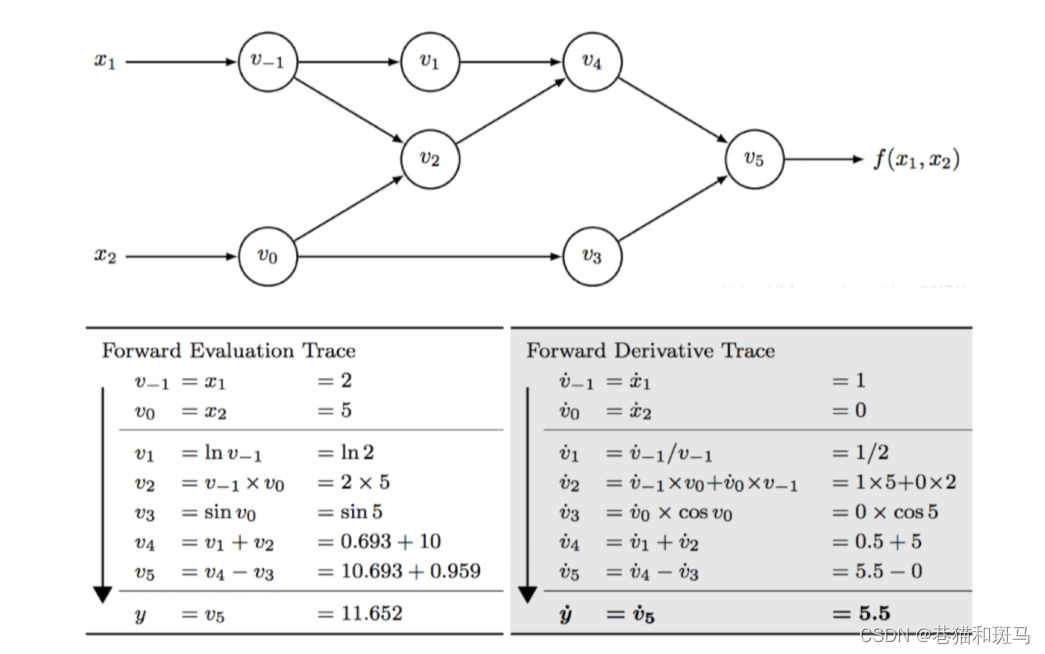
利用有向无环图来表示算术表达式，之后利用该计算图可以实现自动求导，具体效果如下：
在这里插入图片描述
有了tensor，我们可以方便进行深度学习中框架的搭建，即将待处理数据转换为张量，针对张量施加各种需要的操作，通过自动微分对模型展开训练，然后得到输出结果开始测试。

但这里存在一个缺点，由于计算图的维护以及深度学习本身要处理的数据量庞大，tensor的计算速度缓慢。
所以需要扩展包来进行加速，而pytorch可以很好地实现这一功能。同时pytorch也为我们提供了数据加载器等功能，在后面具体进行介绍。

总结：tensro维护了计算图，方便自动求导；pytorch通过利用gpu加速tensor的计算；所以，我们要学习pytorch。tensroflow也是一个常用的加速框架，它常用在工业邻域。

一、基本概念

tensor的三个属性;

rank： tensor的维度
shape：形状
type：tensor的数据类型

tensor的具体操作：

类型的转换
数值操作：按指定类型与形状生成张量
形状变换：变换形状、插入维度、删除维度
数据操作：求和、减法
矩阵的相关操作：反转、矩阵乘法、求行列式

二、基本数据处理与计算操作

1. torch的数据类型

只有float类型可以计算梯度，且torch.Tensor的默认类型为float32
对于数据类型这部分，一般使用默认的数据类型即可。

(1) 查看数据类型

import torch
print(torch.tensor([1,2,3]).dtype)   # 相当于利用数组[1,2,3]创建，所以类型与原数组相同
print(torch.Tensor([1,2,3]).dtype)   # Tensor默认为float32

output:
torch.int64
torch.float32

(2) 改变数据类型

a = torch.tensor([1,2,3])
a = a.float()
print(a.dtype)

a = torch.tensor([1,2,3],dtype=torch.float32)
print(a.dtype)

output:
torch.float32
torch.float32

2. 创建张量

(1) 利用torch提供的函数生成张量

函数	功能
torch.Tensor	基本构造，使用默认类型
torch.tensor	将数组类型转换为tensor
torch.ones	全1
torch.zeros	全0
torch.eye	对角矩阵
torch.rand/randn	均匀/标准正态分布
torch.arange(a,b,step)	从a到b，步长为step
torch.linspace(start,end,steps)	生成从start到end的steps个等间隔向量
torch.normal	正态分布

例子

import torch

# 参数类型：dtype  requires_grad(指定是否要进行梯度计算)
a = torch.tensor((1,2,3),dtype=torch.float,requires_grad=True)

# 标准正态分布:大小为3x3
print(torch.rand(3,3))

# 正态分布
torch.manual_seed(10)   # 设置随机数种子，可以保证程序每次运行生成相同的随机数
# 生成一个均值为0，标准差为1的张量
print(torch.normal(mean=0.0, std = torch.tensor(1.0)))
# 生成一个均值为0，标准差为1，大小为3,3的张量
print(torch.normal(mean=0.0, std = torch.ones(3,3)))

output:
tensor(-1.7029)
tensor([[-0.2653, -0.4747,  0.9289],
        [-0.9621, -0.3161, -0.5910],
        [ 0.4725, -0.3257, -0.5393]])

(2) 利用已有的张量的性质

xxx_like()：生成与指定张量维数相同、性质相同的张量

其中xxx就是上述的zeros、ones

a = torch.tensor((1,2,3),dtype=torch.float,requires_grad=True)
b = torch.zeros_like(a)
print(b)

output:
tensor([0., 0., 0.])

new_xxx()：生成与指定张量性质相似的张量，这个大小可以不同

import torch
a = torch.tensor((1,2,3),dtype=torch.float,requires_grad=True)
c = a.new_tensor([4,5,6])
print(c)
d = a.new_zeros(2,3)
print(d)


output:
tensor([4., 5., 6.])
tensor([[0., 0., 0.],
        [0., 0., 0.]])

(3) numpy进行转化

numpy转为tensor

a = np.ones((3,3))
b = torch.as_tensor(a)
c = torch.from_numpy(a)
print(a)
print(b)
print(c)

output:
[[1. 1. 1.]
 [1. 1. 1.]
 [1. 1. 1.]]
tensor([[1., 1., 1.],
        [1., 1., 1.],
        [1., 1., 1.]], dtype=torch.float64)
tensor([[1., 1., 1.],
        [1., 1., 1.],
        [1., 1., 1.]], dtype=torch.float64)

tensor转为numpy

之所以要进行这个操作，是因为有时我们不需要计算图，通过tensor转numpy，可以节省大量存储空间

a = torch.tensor([1,2,3])
b = a.numpy()
print(b)

output:
[1 2 3]

3. 张量操作

(1) 查看张量的性质

a = torch.tensor([1,2,3])

# 查看维度
print(a.shape)
print(a.size())

# 查看元素的数量
print(a.numel())

(2) 改变张量的形状

tensor.reshape()

a = torch.arange(10.0)
b = a.reshape(2,5)
b = torch.reshape(input=a,shape=(2,-1))
print(a)
print(b)

output:
tensor([0., 1., 2., 3., 4., 5., 6., 7., 8., 9.])
tensor([[0., 1., 2., 3., 4.],
        [5., 6., 7., 8., 9.]])

tensor.resize_()

在torch中，末尾带有_的方法一般是原地操作，即会改变原来元素的形状

c = a.resize_(2,5)
print(a)
print(c)

output:
tensor([[0., 1., 2., 3., 4.],
        [5., 6., 7., 8., 9.]])
tensor([[0., 1., 2., 3., 4.],
        [5., 6., 7., 8., 9.]])

tensor.resize_as_()

如果想要统一两个张量的形状，可以使用这条方法
如果第二个张量的元素个数不等于第一个，则会进行删除或进行0填充

# 第二个张量（待变换）的元素大于第一个
a = torch.arange(12.0).reshape(3,4)
print(a)
b = torch.arange(9).reshape(3,3)
c = a.resize_as_(b)
print(c)

output:
tensor([[0., 1., 2.],
        [3., 4., 5.],
        [6., 7., 8.]])

--------------------------------------------------
# 第二个张量（待变换）元素小于第一个
a = torch.arange(12.0).reshape(3,4)
d = b.resize_as_(a)
print(d)

output:
tensor([[0, 1, 2, 3],
        [4, 5, 6, 7],
        [8, 0, 0, 0]])

torch.view()

view()返回的张量与原来的张量共享内存，修改一个，另一个会跟着改变

x = torch.arange(6.0).reshape(2,3)
y = x.view(6)
z = x.view(-1,2)
print(x.shape,y.shape,z.shape)

output:
torch.Size([2, 3]) torch.Size([6]) torch.Size([3, 2])

如果想要返回拷贝，不与原数据共享内存，可以使用clone

y = x.clone().view(-1,2)

torch.unsqueeze()

在指定的维度插入新的维度

import torch

x = torch.tensor([1, 2, 3, 4])
y = x.unsqueeze(0)  # 在第0维插入一个维度
print(y)  # 输出: tensor([[1, 2, 3, 4]])
print(y.shape)  # 输出: torch.Size([1, 4])

z = x.unsqueeze(1)  # 在第1维插入一个维度
print(z)  # 输出: tensor([[1],
         #              [2],
         #              [3],
         #              [4]])
print(z.shape)  # 输出: torch.Size([4, 1])

torch.squeeze()

移除指定或维度大小为1的维度

a = torch.arange(12.0).reshape(3,4)
b = torch.unsqueeze(a,dim=1)
c = torch.squeeze(b,dim=1)
print(a.size())
print(b.size())
print(c.size())

output:
torch.Size([3, 4])
torch.Size([3, 1, 4])
torch.Size([3, 4])



a = torch.arange(12.0).reshape(1,12)
b = torch.squeeze(a)
print(a.size())
print(b.size())

output:
torch.Size([1, 12])
torch.Size([12])

A.expand()

unsqueeze 用于在张量中插入一个新的维度，而 expand 用于扩展张量的某个维度到更大的尺寸

x = torch.tensor([[1, 2, 3, 4]]) # 大小为(4)
y = x.expand(2, 4)  # 将第0维从1扩展到2,扩展为(2,4)
print(y)  # 输出: tensor([[1, 2, 3, 4],
         #              [1, 2, 3, 4]])
print(y.shape)  # 输出: torch.Size([2, 4])

z = x.expand(4, 1)  # 将第1维从4扩展到1
print(z)  # 输出: tensor([[1],
          #              [2],
          #              [3],
          #              [4]])
print(z.shape)  # 输出: torch.Size([4, 1])

A.expand_as()

将张量扩展到与指定张量同样的大小

a = torch.arange(12.0).reshape(4,3)
b = torch.tensor([1,2,3])
c = b.expand_as(a)
print(c)

output:
tensor([[1, 2, 3],
        [1, 2, 3],
        [1, 2, 3],
        [1, 2, 3]])

A.repeat()

指定每个维度扩展的次数

a = torch.arange(6.0).reshape(2,3)
print(a.repeat(1,2))
print(a.repeat(2,1))
print(a.repeat(2,2))

output:
tensor([[0., 1., 2., 0., 1., 2.],
        [3., 4., 5., 3., 4., 5.]])
tensor([[0., 1., 2.],
        [3., 4., 5.],
        [0., 1., 2.],
        [3., 4., 5.]])
tensor([[0., 1., 2., 0., 1., 2.],
        [3., 4., 5., 3., 4., 5.],
        [0., 1., 2., 0., 1., 2.],
        [3., 4., 5., 3., 4., 5.]])

(3) 获取张量中的元素

索引法

a = torch.arange(12.0).reshape(1,3,4)
print(a)
print(a[0])
print(a[0][0])
print(a[0,0:2,:])
print(a[0,-1,-4:-1])

output:
tensor([[[ 0.,  1.,  2.,  3.],
         [ 4.,  5.,  6.,  7.],
         [ 8.,  9., 10., 11.]]])
tensor([[ 0.,  1.,  2.,  3.],
        [ 4.,  5.,  6.,  7.],
        [ 8.,  9., 10., 11.]])
tensor([0., 1., 2., 3.])
tensor([[0., 1., 2., 3.],
        [4., 5., 6., 7.]])
tensor([ 8.,  9., 10.])

需要注意的是，索引出来的结果与原数据共享内存，修改一个，会影响另一个，

x = torch.arange(6.0).reshape(2,3)
print(x)
y = x[0,:]
y += 1
print(y)
print(x)

output:
tensor([[0., 1., 2.],
        [3., 4., 5.]])
tensor([1., 2., 3.])
tensor([[1., 2., 3.],
        [3., 4., 5.]])

如果想要使得修改不互相影响，可以使用clone()

x = torch.arange(6.0).reshape(2,3)
z = x[0,:].clone()
print(x)
z += 1
print(x)

output:
tensor([[0., 1., 2.],
        [3., 4., 5.]])
tensor([[0., 1., 2.],
        [3., 4., 5.]])

条件筛选

类似于c中的条件判断语句

a = torch.arange(12.0).reshape(3,4)
b = -a
c = torch.where(a>3,a,b)
print(c)

output:
tensor([[-0., -1., -2., -3.],
        [ 4.,  5.,  6.,  7.],
        [ 8.,  9., 10., 11.]])

(4) 拼接

cat 用于在已有的维度上连接张量，而 stack 用于在新的维度上堆叠张量。cat 不改变张量的总维度，而 stack 会增加一个新的维度。

torch.cat

torch.cat 函数用于在给定的维度上连接两个或多个张量。这个操作要求所有张量在除连接维度外的其他维度上具有相同的形状。连接维度上的大小可以不同，cat 会将它们按顺序排列。

cat会在已有的维度上进行融合，在深度学习中需要进行特征图的特征融合时，通常会用到

import torch

x = torch.tensor([1, 2, 3])
y = torch.tensor([4, 5, 6])

z = torch.cat((x, y), 0)  # 在第0维上连接x和y
print(z)  # 输出: tensor([1, 2, 3, 4, 5, 6])
print(z.size())

output:
tensor([1, 2, 3, 4, 5, 6])
torch.Size([6])

torch.stack

stack类似于将两个张量堆叠在一起，它会增加一个新的维度。
在深度学习的用途：我们有时会遇到三元组样本的对比操作，需要将锚样本分别与正负样本打包在一起，这时就可以使用stack来实现，这个大家现在理解可能会比较难，等到实验遇到具体操作会豁然开朗。

import torch
a = torch.tensor([1,2,3])
b = torch.tensor([4,5,6])
c = torch.stack((a,b),0)
d = torch.stack((a,b),1)

print(a.size())
print(b.size())
print(c.size())
print(d.size())


output:
torch.Size([3])
torch.Size([3])
torch.Size([2, 3])
torch.Size([3, 2])

总结： cat类似于融合，stack类似于打包

(5) 拆分

torch.chunk
沿着dim维度，分为两块，不能整除的话最后一块最小

A = torch.arange(10).reshape(2, 5)
D1, D2, D3 = torch.chunk(A, 3, dim=1)
print(D1)
print(D2)
print(D3)

>>>tensor([[0, 1],
           [5, 6]])
>>>tensor([[2, 3],
           [7, 8]])
>>>tensor([[4],
           [9]])

torch.split
将张量分块，可以指定每一块的大小

A = torch.arange(12).reshape(2, 6)
'''按照维度1分为三块，大小分别为1，2，3'''
D1, D2, D3 = torch.split(A, [1, 2, 3], dim=1)
print(D1)
print(D2)
print(D3)

>>>tensor([[0],
          [6]])
>>>tensor([[1, 2],
           [7, 8]])
>>>tensor([[ 3,  4,  5],
           [ 9, 10, 11]])

4. 张量计算

(1) 加法

两个不同的张量求和

x + y

torch.add(x+y)
# 原地操作
y.add_(x)

同一个张量中的元素求和

x = torch.arange(6.0).reshape(2,3)
print(x)
# 第二维元素求和
print(sum(x))
# 所有元素求和
print(torch.sum(x))
print(x.sum())

output:
tensor([[0., 1., 2.],
        [3., 4., 5.]])
tensor([3., 5., 7.])
tensor(15.)

(2) 乘法

对应位置元素相乘

a = torch.tensor([1, 2, 3], dtype=torch.float32)
b = torch.tensor([4, 5, 6], dtype=torch.float32)
dot_product = a * b
print(dot_product)


output:
tensor([ 4., 10., 18.])

点积

import torch

a = torch.tensor([1, 2, 3], dtype=torch.float32)
b = torch.tensor([4, 5, 6], dtype=torch.float32)
dot_product = torch.dot(a, b)

output:
tensor(32.)

矩阵乘法

A = torch.tensor([[1, 2], [3, 4]], dtype=torch.float32)
B = torch.tensor([[5, 6], [7, 8]], dtype=torch.float32)
matrix_multiply = torch.matmul(A, B)

(3) 比较

torch.eq()

判断两个元素是否相等

A = torch.tensor([1,2,3,4,5,6])
B = torch.arange(1,7)
C = torch.unsqueeze(B,dim=0)
print(torch.eq(A,B))
print(torch.eq(A,C))

>>>tensor([True, True, True, True, True, True])
>>>tensor([[True, True, True, True, True, True]])

torch.equal()

判断两个张量形状和元素是否相同

A = torch.tensor([1,2,3,4,5,6])
B = torch.arange(1,7)
C = torch.unsqueeze(B,dim=0)
print(torch.equal(A,B))
print(torch.equal(A,C))

>>>True
>>>False

torch.isnan()

判断是否为缺失值

print(torch.isnan(torch.tensor([0,1,float("nan"),2])))

>>>tensor([False, False,  True, False])

(4) 广播机制

当对两个形状不同的tensor按照元素运算时，可能会触发广播机制：改变两个元素的大小，使得每一维都扩展到两个张量中最大的那个，eg：[1,2]+[2,1]扩展为[2,2]

x = torch.arange(2.0).view(1,2)
y = torch.arange(3.0).view(3,1)
print(x)
print(y)
print(x+y)

output:
tensor([[0., 1.]])
tensor([[0.],
        [1.],
        [2.]])
tensor([[0., 1.],
        [1., 2.],
        [2., 3.]])

(5) 使用gpu运算

首先要有gpu版本的torch

x = torch.arange(6.0).reshape(2,3)

if torch.cuda.is_available():
	device = torch.device("cuda")
	y = torch.ones_like(x,device=device)
	x = x.to(device)
	z = x+y
	print(z)
	print(z.to("cpu",torch.float64))

(6) 自动求梯度

grad_fn
在tensor中，利用Tensor和Function相互结合可以构建一个记录有整个计算过程DAG。我们通过这个DAG图来实现梯度计算。每个tensor本身有一个grad_fn属性。
Function的创建就是由tensor中的grad_fn维护的，如果该tensor是由某些运算得到（即有DAG图），则grad_fn返回一个与这些运算有关的对象，否则就是None。

创建得到的张量

x = torch.ones(2,2,requires_grad=True)
print(x)
print(x.grad_fn)

output:
tensor([[1., 1.],
        [1., 1.]], requires_grad=True)
None

计算得到的张量

y = x+1
print(y)
print(y.grad_fn)

output:
tensor([[2., 2.],
        [2., 2.]], grad_fn=<AddBackward0>)
<AddBackward0 object at 0x00000172D9331488>

修改梯度性质

x = torch.ones(2,2)
print(x.requires_grad)
x.requires_grad_(True)
print(x.requires_grad)

output:
False
True

梯度计算

x = torch.ones(2,2,requires_grad=True)
y = x+2
z = y*y*3
out = z.mean()
out.backward()

print(x.grad)

output:
tensor([[4.5000, 4.5000],
        [4.5000, 4.5000]])

上述计算式为：
$\frac{1}{4} \sum_{i=1}^4z_i = \frac{1}{4}\sum_{i=1}^43(x_i+2)^2$

默认情况下，梯度是累加的

x = torch.ones(2,2,requires_grad=True)
y = x+2
z = y*y*3
out = z.mean()
out.backward()

print(x.grad)

out2 = x.sum()
out2.backward()
print(x.grad)

out3 = x.sum()
x.grad.data.zero_()  # 梯度清零
out3.backward()
print(x.grad)

output:
tensor([[4.5000, 4.5000],
        [4.5000, 4.5000]])
tensor([[5.5000, 5.5000],
        [5.5000, 5.5000]])
tensor([[1., 1.],
        [1., 1.]]

net中的梯度清零

我的毕设中的一个例子，大家只要记住
network.zero_grad()即可

loss_p = torch.sum(torch.clamp(torch.add(torch.div(relation_pos, -1), (alp + margin), out=None), min=0))
            # r - (a-m)，如果r<a-m，则损失为0
            # 损失相乘操作加权重 label
loss_n = torch.sum(torch.mul(relation_neg, torch.clamp(relation_neg - (alp - margin), min=0)))

loss = loss_p + loss_n

feature_encoder.zero_grad()
loss.backward()

取消自动梯度计算
在评估阶段，我们不需要进行梯度的反向传播，可以通过以下方式：

import torch

# 假设我们有一个模型和一个输入张量
model = ...  # 你的模型
input_data = ...  # 你的输入数据

# 在评估模式下设置模型
model.eval()

# 使用 with torch.no_grad() 来包裹不需要计算梯度的代码
with torch.no_grad():
    # 在这里执行的代码不会计算梯度
    output = model(input_data)
    # ... 可以执行其他操作，比如计算损失函数等

张量求导的要求

在我们利用out.backward()进行梯度的计算时，我们要明确out是标量还是张量，如果是张量，则需要我们在backward()中传入一个与out同形的张量，保证是标量out对张量x求导。
如果不这样做，则根据张量对张量的求导法则，最终会计算得出一个高维张量，对于高维张量，我们的计算是非常困难的。

x = torch.tensor([1.0,2.0,3.0,4.0],requires_grad=True)
y = 2*x
z = y.view(2,2)
print(z)
v = torch.tensor([[1.0,0.1],[0.01,0.001]],dtype=torch.float)
z.backward(v) # 底层进行了 (z*v).sum()计算得到一个标量
print(x.grad)

output:
tensor([2.0000,0.2000,0.0200,0.0020])