Asset Pricing：Expected Utility Theory

Asset Pricing：Expected Utility Theory

Theorem 1（Represention Theorem）：Suppose the preference ordering is :

1. complete
2. transitive
3. continuous

then the preference ordering can be represented by a utility function, that is, $c\succ c^{\prime }$ iff $\exists u(\cdot ),s.t.u(c)>u(c^{\prime })$​​.

经典的效用函数表示定理

Expected Utility (冯诺依曼——摩根斯坦)：

We define the (finite) set of outcomes $X$ and we define a lottery as a probability measure over $X$, that is a function $p:X\in [0,1]$ such that

1. for $x\in X,p(x)\ge 0$
2. ${\sum }_{x\in X}p(x)=1$

The set of all possible lotteries is：
P ≡ { p : X → [ 0 , 1 ] ∣ ∀ x ∈ X , p ( x ) ≥ 0 , ∑ x ∈ X p ( x ) = 1 } P\equiv\{p:X\to[0,1]|\forall x\in X,p(x)\geq0,\sum_{x\in X}p(x)=1\} P≡{p:X→[0,1]∣∀x∈X,p(x)≥0,x∈X∑​p(x)=1}
Assume there exists a preference relation $\succ$​ over P.

Von Neumann - Morgenstern Axioms:

1. Regularity: preference $\succ$ is complete and transitive
2. Independence: For any $p,q,r\in P,\alpha \in [0,1],p⪰q\iff \alpha p+(1-\alpha )r⪰\alpha q+(1-\alpha )r$
3. Continuity: For any $p,q,r\in P$​ , if $p\succ q\succ r,\exists \alpha ,\beta \in (0,1),s.t.\alpha p+(1-\alpha )r>q>\beta p+(1-\beta )r$​​

Theorem (Expected Utility Representation)：If a preference relation $\succ$ over $P$ satisfies the Regularity, Independence and Continuity axioms, then there exists a function $u$ : $X\to \mathbb{R}$​ such that
$$p⪰q\iff \sum _{x\in X}p(x)u(x)\ge \sum _{x\in X}q(x)u(x)$$

Risk Aversion, Concavity, Certainty Equivalent

Consider a lottery $p$ with possible outcomes $x_0<x_1$.

Certainty Equivalent: the certain payoff which gives the same expected utility as the uncertain lottery $p$.

If $\mathbb{E}[u(x)]\to$ expected utility of lottery $p$, then $u^{-1}(\mathbb{E}[u(x)])\to$ CE of $p$.

suppose that the agent is risk-averse: $u^{-1}(\mathbb{E}[u(x)])<\mathbb{E}[x]\iff u(\cdot )$​ is concave, because:
$$\begin{gathered} u^{-1}(\mathbb{E}[u(x)])<\mathbb{E}[x] \\ \mathbb{E}[u(x)]<u(\mathbb{E}[x]) \end{gathered}$$

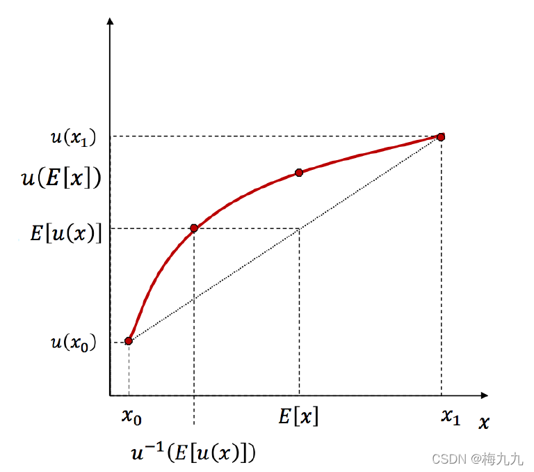
the difference $\mathbb{E}[x]-u^{-1}(\mathbb{E}[u(x)])$​​ is called Risk Premium.

Risk Aversion : $u^{-1}(\mathbb{E}[u(x)])<\mathbb{E}(x)$​

Risk loving : $u^{-1}(\mathbb{E}[u(x)])>\mathbb{E}(x)$​

Risk neutral : $u^{-1}(\mathbb{E}[u(x)])=\mathbb{E}(x)$​

Risk-Attitude $\iff$​ concavity of $u(\cdot )$​

Theorem 1: Let $F_A$​ and $F_B$​ be two CDFs for the random payoffs $x\in [a,b]$​. Then $F_A$​ FOSD $F_B$​ if and only if ${\mathbb{E}}_A[U(x)]\ge {\mathbb{E}}_B[U(x)]$​ for all nondecreasing utility functions $U(\cdot )$​​​.

Theorem 2: Let $F_A$​ and $F_B$​ be two CDFs for the random payoffs $x\in [a,b]$​. Then $F_A$​ SOSD $F_B$​ if and only if ${\mathbb{E}}_A[U(x)]\ge {\mathbb{E}}_B[U(x)]$​ for all nondecreasing and concave utility functions $U(\cdot )$​.

1. 经典效用函数理论：suppose $U(c)=U(c_0,c_1,\cdots ,c_S)$​ represent a complete, transitive and continuous preference ordering between consumption profiles. Then also $V(c)=f(U(c))$, for $f$ strictly increasing, represents the same preference ordering.
2. Expected Utility function：suppose that $\mathbb{E}[u(c)]$​ represents a preference ordering satisfying the Von Neumann-Morgenstern axioms. Then for $a,b\in \mathbb{R}$​ the affine function $v(c)=a+bu(c)$​ , $\mathbb{E}[u(c)]$​ and $\mathbb{E}[v(c)]$​ represent the same preference ordering.

Measures of Risk Aversion

1. Absolute Risk Aversion：$R_A(Y)=-\frac{u^{\prime \prime }(Y)}{u^{\prime }(Y)}$​​
2. Relative Risk Aversion：$R_R(Y)=-Y\frac{u^{\prime \prime }(Y)}{u^{\prime }(Y)}=Y\cdot R_A(Y)$
3. Risk Tolerance：$R_T(Y)=\frac{1}{R_A(Y)}$

two specific functional forms for the Von Neumann-Morgenstern function $U$：

1. Constant Absolute Risk Aversion (CARA) utility function：$U(x)=-e^{\rho x},\rho >0$
2. Constant Relative Risk Aversion (CRRA) utility function：$U(x)=\{\begin{array}{l}\frac{x^{1-\gamma }}{1-\gamma },if\gamma \ne 1\\ \ln x,if\gamma =1\end{array}$​

Risk Aversion and Portfolio Allocation

Assume two assets, one is risky with random net return $r$​ , one is risk-free with net return $r^f$​ , Initial wealth is $Y_0$​ .We want to maximize the expected utility by choosing the risky asset allocation parameter $a\in R$​：
$$\underset{a\in R}{\max }E[U(Y_0(1+r^f)+a(r-r^f))]$$
FOC：
$$E[U^{\prime }(Y_0(1+r^f)+a(r-r^f))(r-r^f)]=0$$
We can characterize the solution to the problem with the following theorem:

Theorem : assume $U^{\prime }>0,U^{\prime \prime }<0$ and let $\hat{a}$ denote the solution to the problem above. Then :
$$\begin{gathered} \hat{a}>0\iff \mathbb{E}[r]>r^f \\ \hat{a}=0\iff \mathbb{E}[r]=r^f \\ \hat{a}<0\iff \mathbb{E}[r]<r^f \end{gathered}$$

proof : define $W(a)\equiv \mathbb{E}[U(Y_0(1+r^f)+a(r-r^f))]$, then FOC $\to$ $W^{\prime }(a)=0$

risk aversion $\to U^{\prime }>0,U^{\prime \prime }<0\to W^{\prime \prime }(a)=E[U^{\prime \prime }(Y_0(1+r^f)+a(r-r^f))(r-r^f{)}^2]<0$

so $W^{\prime }(a)$​​ is everywhere decreasing in $a$.

So $\hat{a}>0$ iff $W^{\prime }(0)>0$, since $U^{\prime }>0$ if follows that $\hat{a}>0$ iff $\mathbb{E}[r]>r^f$.

其他证明类似。

Arrow’s theorem :

Theorem 1 : Let $\hat{a}=\hat{a}(Y_0)$​ be the solution to the problem above, then :
$$\begin{gathered} \frac{\partial R_A}{\partial Y_0}<0\to \frac{\partial \hat{a}}{\partial Y_0}>0 \\ \frac{\partial R_A}{\partial Y_0}=0\to \frac{\partial \hat{a}}{\partial Y_0}=0 \\ \frac{\partial R_A}{\partial Y_0}>0\to \frac{\partial \hat{a}}{\partial Y_0}<0 \end{gathered}$$

Theorem 2 : If , for all wealth levels $Y$ :
$$\begin{gathered} \frac{\partial R_R}{\partial Y_0}<0\to \frac{da/a}{dY/Y}>1 \\ \frac{\partial R_R}{\partial Y_0}=0\to \frac{da/a}{dY/Y}=1 \\ \frac{\partial R_R}{\partial Y_0}>0\to \frac{da/a}{dY/Y}<1 \end{gathered}$$

In the special case $U(Y)=\ln Y$​ the FOC is
$$\mathbb{E}[\frac{r-r^f}{Y_0(1+r^f)+a(r-r^f)}]=0$$
assuming that $r$​​ can take on two possible values $r_1,r_2,r_1<r^f<r_2$​​, it is possible to show that :
$$\frac{a}{Y_0}=\frac{(1+r^f)(E[r]-r^f)}{(r_2-r^f)(r^f-r_1)}>0$$

Theorem (Cass and Stiglitz): Let the vector
$$\left[\begin{array}{c}{\hat{a}}_1(Y_0)\\ ⋮\\ {\hat{a}}_J(Y_0)\end{array}\right]$$
denote the amount optimally invested in the $J$ risky assets if the initial wealth is $Y_0$​, then:
$$\left[\begin{array}{c}{\hat{a}}_1(Y_0)\\ ⋮\\ {\hat{a}}_J(Y_0)\end{array}\right]=\left[\begin{array}{c}{\hat{a}}_1\\ ⋮\\ {\hat{a}}_J\end{array}\right]\cdot f(Y_0)$$
if and only if either i)$U^{\prime }(Y_0)=(\theta Y_0+k{)}^{\Delta }$ or ii)$U^{\prime }(Y_0)=\xi e^{-v{Y}_0}$

To conclude this subsection, we generalize the class of utility functions by starting from the absolute risk aversion (and then backing out the resulting utility function).

We call linear risk tolerance (or hyperbolic risk aversion) any utility function such that
$$R_A=-\frac{u^{\prime \prime }(c)}{u^{\prime }(c)}=\frac{1}{A+B\cdot c}$$
Clearly, for $B=0$ and $A\ne 0$ we have a CARA utility function. If $B\ne 0$​​ we obtain a generalized power function
$$u(c)=\frac{1}{B-1}(A+B\cdot c{)}^{\frac{B-1}{B}}$$

if $B\to 1$​ :（洛必达）
$$\begin{gathered} u(c)=\underset{B\to 1}{\lim }\frac{(A+B\cdot c{)}^{\frac{B-1}{B}}}{B-1} \\ =\underset{B\to 1}{\lim }\frac{(A+B\cdot c{)}^{\frac{B-1}{B}}\ln (A+B\cdot c)}{1} \\ =\ln (A+B\cdot c) \end{gathered}$$
for $B=-1$​​ we obtain quadratic utility $-\frac{1}{2}(A-c{)}^2$​​, and for $A=0$​​ we obtain the CRRA utility function $u(c)=\frac{1}{B-1}(B\cdot c{)}^{\frac{B-1}{B}}$​​.

Savings

Let’s jump forward a little and suppose that in a multi-period setting agents maximize the expected utility :
$${\mathbb{E}}_0[\sum _{t=0}^{\infty }{\beta }^{t}u(c_t)]$$
subject to the intertemporal budget constraint
$$c_{t+1}=e_{t+1}+(1+r)(e_t-c_t)$$
The standard Euler equation is
$$u^{\prime }(c_t)=\beta (1+r){\mathbb{E}}_t[u^{\prime }(c_{t+1})]$$
if $u^{\prime \prime \prime }>0$ , Jensen’s nequality implies:
$$\frac{1}{\beta (1+r)}=\frac{{\mathbb{E}}_t[u^{\prime }(c_{t+1})]}{u^{\prime }(c_t)}>\frac{u^{\prime }({\mathbb{E}}_t[c_{t+1}])}{u^{\prime }(c_t)}$$
Which shows that the marginal rate of intertemporal substitution is higher in the presence of uncertainty in $c_{t+1}$​. The difference between the two marginal rates, with and without uncertainty, is attributed to precautionary savings. to see this, suppose the variance of $e_{t+1}$ increases (in a mean preserving fashion). Since numerator ${\mathbb{E}}_t[u^{\prime }(c_{t+1})]$ is increasing in the variance of $c_{t+1}$, in order for the above equality to hold $c_t$ must decrease, that is, savings increase due to precautionary savings.