【脉搏信号分析】脉搏波PPG信号分析附Matlab代码

✅作者简介：热爱科研的Matlab仿真开发者，擅长数据处理、建模仿真、程序设计、完整代码获取、论文复现及科研仿真。

🍎个人主页：Matlab科研工作室

🍊个人信条：格物致知,完整Matlab代码及仿真咨询内容私信。

🌿 往期回顾可以关注主页，点击搜索

🔥 内容介绍

脉搏波（PPG）信号是一种重要的生理信号，它反映了心脏的活动和血管系统的状态。PPG信号分析在医学诊断和健康监测中有着广泛的应用。本文将介绍PPG信号分析的基本原理、方法和应用。

PPG信号的产生

PPG信号是由心脏搏动引起的血管体积变化产生的。当心脏收缩时，血液被泵入动脉，导致动脉扩张，从而产生一个PPG信号峰值。当心脏舒张时，动脉收缩，PPG信号下降。

PPG信号特征

PPG信号具有以下特征：

• **峰值：**对应于心脏收缩。

• **波谷：**对应于心脏舒张。

• **上升时间：**从波谷到峰值的持续时间。

• **下降时间：**从峰值到波谷的持续时间。

• **心率：**峰值之间的间隔。

PPG信号分析方法

PPG信号分析通常涉及以下步骤：

• **预处理：**去除噪声和其他干扰。

• **特征提取：**提取PPG信号的特征，如峰值、波谷、心率等。

• **分类：**根据PPG信号特征将信号分类为正常或异常。

• **解释：**解释PPG信号特征的生理意义。

PPG信号分析的应用

PPG信号分析在医学诊断和健康监测中有着广泛的应用，包括：

• **心血管疾病诊断：**检测心律失常、心力衰竭和冠状动脉疾病等心血管疾病。

• **呼吸系统疾病诊断：**检测睡眠呼吸暂停和慢性阻塞性肺病等呼吸系统疾病。

• **健康监测：**监测心率、血压和血氧饱和度等健康指标。

• **运动生理学：**评估运动时的生理反应。

• **远程医疗：**通过可穿戴设备远程监测患者的健康状况。

结论

PPG信号分析是一种强大的工具，可用于诊断疾病、监测健康和评估生理反应。随着传感器技术和数据分析方法的不断发展，PPG信号分析在医学和健康保健领域将发挥越来越重要的作用。

📣 部分代码

%EMD  computes Empirical Mode Decomposition%%%   Syntax%%% IMF = EMD(X)% IMF = EMD(X,...,'Option_name',Option_value,...)% IMF = EMD(X,OPTS)% [IMF,ORT,NB_ITERATIONS] = EMD(...)%%%   Description%%% IMF = EMD(X) where X is a real vector computes the Empirical Mode% Decomposition [1] of X, resulting in a matrix IMF containing 1 IMF per row, the% last one being the residue. The default stopping criterion is the one proposed% in [2]:%%   at each point, mean_amplitude < THRESHOLD2*envelope_amplitude%   &%   mean of boolean array {(mean_amplitude)/(envelope_amplitude) > THRESHOLD} < TOLERANCE%   &%   |#zeros-#extrema|<=1%% where mean_amplitude = abs(envelope_max+envelope_min)/2% and envelope_amplitude = abs(envelope_max-envelope_min)/2% % IMF = EMD(X) where X is a complex vector computes Bivariate Empirical Mode% Decomposition [3] of X, resulting in a matrix IMF containing 1 IMF per row, the% last one being the residue. The default stopping criterion is similar to the% one proposed in [2]:%%   at each point, mean_amplitude < THRESHOLD2*envelope_amplitude%   &%   mean of boolean array {(mean_amplitude)/(envelope_amplitude) > THRESHOLD} < TOLERANCE%% where mean_amplitude and envelope_amplitude have definitions similar to the% real case%% IMF = EMD(X,...,'Option_name',Option_value,...) sets options Option_name to% the specified Option_value (see Options)%% IMF = EMD(X,OPTS) is equivalent to the above syntax provided OPTS is a struct % object with field names corresponding to option names and field values being the % associated values %% [IMF,ORT,NB_ITERATIONS] = EMD(...) returns an index of orthogonality%                       ________%         _  |IMF(i,:).*IMF(j,:)|%   ORT = \ _____________________%         /%         ?       || X ||?%        i~=j%% and the number of iterations to extract each mode in NB_ITERATIONS%%%   Options%%%  stopping criterion options:%% STOP: vector of stopping parameters [THRESHOLD,THRESHOLD2,TOLERANCE]% if the input vector's length is less than 3, only the first parameters are% set, the remaining ones taking default values.% default: [0.05,0.5,0.05]%% FIX (int): disable the default stopping criterion and do exactly <FIX> % number of sifting iterations for each mode%% FIX_H (int): disable the default stopping criterion and do <FIX_H> sifting % iterations with |#zeros-#extrema|<=1 to stop [4]%%  bivariate/complex EMD options:%% COMPLEX_VERSION: selects the algorithm used for complex EMD ([3])% COMPLEX_VERSION = 1: "algorithm 1"% COMPLEX_VERSION = 2: "algorithm 2" (default)% % NDIRS: number of directions in which envelopes are computed (default 4)% rem: the actual number of directions (according to [3]) is 2*NDIRS% %  other options:%% T: sampling times (line vector) (default: 1:length(x))%% MAXITERATIONS: maximum number of sifting iterations for the computation of each% mode (default: 2000)%% MAXMODES: maximum number of imfs extracted (default: Inf)%% DISPLAY: if equals to 1 shows sifting steps with pause% if equals to 2 shows sifting steps without pause (movie style)% rem: display is disabled when the input is complex%% INTERP: interpolation scheme: 'linear', 'cubic', 'pchip' or 'spline' (default)% see interp1 documentation for details%% MASK: masking signal used to improve the decomposition according to [5]%%%   Examples%%%X = rand(1,512);%%IMF = emd(X);%%IMF = emd(X,'STOP',[0.1,0.5,0.05],'MAXITERATIONS',100);%%T=linspace(0,20,1e3);%X = 2*exp(i*T)+exp(3*i*T)+.5*T;%IMF = emd(X,'T',T);%%OPTIONS.DISLPAY = 1;%OPTIONS.FIX = 10;%OPTIONS.MAXMODES = 3;%[IMF,ORT,NBITS] = emd(X,OPTIONS);%%%   References%%% [1] N. E. Huang et al., "The empirical mode decomposition and the% Hilbert spectrum for non-linear and non stationary time series analysis",% Proc. Royal Soc. London A, Vol. 454, pp. 903-995, 1998%% [2] G. Rilling, P. Flandrin and P. Gon鏰lves% "On Empirical Mode Decomposition and its algorithms",% IEEE-EURASIP Workshop on Nonlinear Signal and Image Processing% NSIP-03, Grado (I), June 2003%% [3] G. Rilling, P. Flandrin, P. Gon鏰lves and J. M. Lilly.,% "Bivariate Empirical Mode Decomposition",% Signal Processing Letters (submitted)%% [4] N. E. Huang et al., "A confidence limit for the Empirical Mode% Decomposition and Hilbert spectral analysis",% Proc. Royal Soc. London A, Vol. 459, pp. 2317-2345, 2003%% [5] R. Deering and J. F. Kaiser, "The use of a masking signal to improve % empirical mode decomposition", ICASSP 2005%%% See also%  emd_visu (visualization),%  emdc, emdc_fix (fast implementations of EMD),%  cemdc, cemdc_fix, cemdc2, cemdc2_fix (fast implementations of bivariate EMD),%  hhspectrum (Hilbert-Huang spectrum)%%% G. Rilling, last modification: 3.2007% gabriel.rilling@ens-lyon.fr​​function [imf,ort,nbits] = emd(varargin)​[x,t,sd,sd2,tol,MODE_COMPLEX,ndirs,display_sifting,sdt,sd2t,r,imf,k,nbit,NbIt,MAXITERATIONS,FIXE,FIXE_H,MAXMODES,INTERP,mask] = init(varargin{:});​if display_sifting  fig_h = figure;end​​%main loop : requires at least 3 extrema to proceedwhile (~stop_EMD(r,MODE_COMPLEX,ndirs) && (k < MAXMODES+1 || MAXMODES == 0) && ~any(mask))​  % current mode  m = r;​  % mode at previous iteration  mp = m;​  %computation of mean and stopping criterion  if FIXE    [stop_sift,moyenne] = stop_sifting_fixe(t,m,INTERP,MODE_COMPLEX,ndirs);  elseif FIXE_H    stop_count = 0;    [stop_sift,moyenne] = stop_sifting_fixe_h(t,m,INTERP,stop_count,FIXE_H,MODE_COMPLEX,ndirs);  else    [stop_sift,moyenne] = stop_sifting(m,t,sd,sd2,tol,INTERP,MODE_COMPLEX,ndirs);  end​  % in case the current mode is so small that machine precision can cause  % spurious extrema to appear  if (max(abs(m))) < (1e-10)*(max(abs(x)))    if ~stop_sift      warning('emd:warning','forced stop of EMD : too small amplitude')    else      disp('forced stop of EMD : too small amplitude')    end    break  end​​  % sifting loop  while ~stop_sift && nbit<MAXITERATIONS    if(~MODE_COMPLEX && nbit>MAXITERATIONS/5 && mod(nbit,floor(MAXITERATIONS/10))==0 && ~FIXE && nbit > 100)      disp(['mode ',int2str(k),', iteration ',int2str(nbit)])      if exist('s','var')        disp(['stop parameter mean value : ',num2str(s)])      end      [im,iM] = extr(m);      disp([int2str(sum(m(im) > 0)),' minima > 0; ',int2str(sum(m(iM) < 0)),' maxima < 0.'])    end​    %sifting    m = m - moyenne;​    %computation of mean and stopping criterion    if FIXE      [stop_sift,moyenne] = stop_sifting_fixe(t,m,INTERP,MODE_COMPLEX,ndirs);    elseif FIXE_H      [stop_sift,moyenne,stop_count] = stop_sifting_fixe_h(t,m,INTERP,stop_count,FIXE_H,MODE_COMPLEX,ndirs);    else      [stop_sift,moyenne,s] = stop_sifting(m,t,sd,sd2,tol,INTERP,MODE_COMPLEX,ndirs);    end​    % display    if display_sifting && ~MODE_COMPLEX      NBSYM = 2;      [indmin,indmax] = extr(mp);      [tmin,tmax,mmin,mmax] = boundary_conditions(indmin,indmax,t,mp,mp,NBSYM);      envminp = interp1(tmin,mmin,t,INTERP);      envmaxp = interp1(tmax,mmax,t,INTERP);      envmoyp = (envminp+envmaxp)/2;      if FIXE || FIXE_H        display_emd_fixe(t,m,mp,r,envminp,envmaxp,envmoyp,nbit,k,display_sifting)      else        sxp=2*(abs(envmoyp))./(abs(envmaxp-envminp));        sp = mean(sxp);        display_emd(t,m,mp,r,envminp,envmaxp,envmoyp,s,sp,sxp,sdt,sd2t,nbit,k,display_sifting,stop_sift)  defopts.display = 0;defopts.t = 1:max(size(x));defopts.maxiterations = 2000;defopts.fix = 0;defopts.maxmodes = 0;defopts.interp = 'spline';defopts.fix_h = 0;defopts.mask = 0;defopts.ndirs = 4;defopts.complex_version = 2;​opts = defopts;​​​if(nargin==1)  inopts = defopts;elseif nargin == 0  error('not enough arguments')end​​names = fieldnames(inopts);for nom = names'  if ~any(strcmpi(char(nom), opt_fields))    error(['bad option field name: ',char(nom)])  end  if ~isempty(eval(['inopts.',char(nom)])) % empty values are discarded    eval(['opts.',lower(char(nom)),' = inopts.',char(nom),';'])  endend​t = opts.t;stop = opts.stop;display_sifting = opts.display;MAXITERATIONS = opts.maxiterations;FIXE = opts.fix;MAXMODES = opts.maxmodes;INTERP = opts.interp;FIXE_H = opts.fix_h;mask = opts.mask;ndirs = opts.ndirs;complex_version = opts.complex_version;​if ~isvector(x)  error('X must have only one row or one column')end​if size(x,1) > 1  x = x.';end​if ~isvector(t)  error('option field T must have only one row or one column')end​if ~isreal(t)  error('time instants T must be a real vector')end​if size(t,1) > 1  t = t';end​if (length(t)~=length(x))  error('X and option field T must have the same length')end​if ~isvector(stop) || length(stop) > 3  error('option field STOP must have only one row or one column of max three elements')end​if ~all(isfinite(x))  error('data elements must be finite')end​if size(stop,1) > 1  stop = stop';end​L = length(stop);if L < 3  stop(3)=defstop(3);end​if L < 2  stop(2)=defstop(2);end​​if ~ischar(INTERP) || ~any(strcmpi(INTERP,{'linear','cubic','spline'}))  error('INTERP field must be ''linear'', ''cubic'', ''pchip'' or ''spline''')end​%special procedure when a masking signal is specifiedif any(mask)  if ~isvector(mask) || length(mask) ~= length(x)    error('masking signal must have the same dimension as the analyzed signal X')  end​  if size(mask,1) > 1    mask = mask.';  end  opts.mask = 0;  imf1 = emd(x+mask,opts);  imf2 = emd(x-mask,opts);  if size(imf1,1) ~= size(imf2,1)    warning('emd:warning',['the two sets of IMFs have different sizes: ',int2str(size(imf1,1)),' and ',int2str(size(imf2,1)),' IMFs.'])  end  S1 = size(imf1,1);  S2 = size(imf2,1);  if S1 ~= S2    if S1 < S2      tmp = imf1;      imf1 = imf2;      imf2 = tmp;    end    imf2(max(S1,S2),1) = 0;  end  imf = (imf1+imf2)/2;​end​​sd = stop(1);sd2 = stop(2);tol = stop(3);​lx = length(x);​sdt = sd*ones(1,lx);sd2t = sd2*ones(1,lx);​if FIXE  MAXITERATIONS = FIXE;  if FIXE_H    error('cannot use both ''FIX'' and ''FIX_H'' modes')  endend​MODE_COMPLEX = ~isreal(x)*complex_version;if MODE_COMPLEX && complex_version ~= 1 && complex_version ~= 2  error('COMPLEX_VERSION parameter must equal 1 or 2')end​​% number of extrema and zero-crossings in residualner = lx;nzr = lx;​r = x;​if ~any(mask) % if a masking signal is specified "imf" already exists at this stage  imf = [];endk = 1;​% iterations counter for extraction of 1 modenbit=0;​% total iterations counterNbIt=0;end%---------------------------------------------------------------------------------------------------​

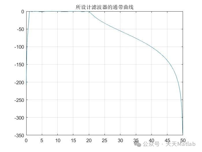
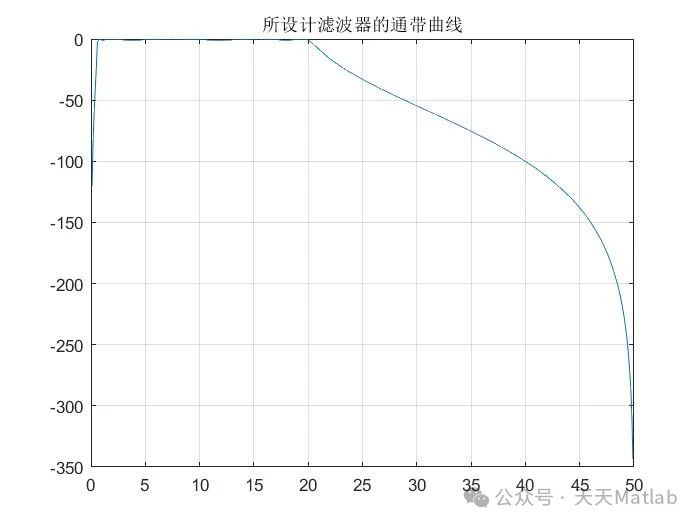
⛳️ 运行结果

🔗 参考文献

[1] 蒋文俊.智能手机脉搏波信号实时检测与分析[D].清华大学,2015.

[2] 蒋文俊.智能手机脉搏波信号实时检测与分析[D].清华大学[2024-02-29].DOI:CNKI:CDMD:2.1015.039039.

🎈 部分理论引用网络文献，若有侵权联系博主删除

🎁  关注我领取海量matlab电子书和数学建模资料

👇  私信完整代码和数据获取及论文数模仿真定制

1 各类智能优化算法改进及应用

生产调度、经济调度、装配线调度、充电优化、车间调度、发车优化、水库调度、三维装箱、物流选址、货位优化、公交排班优化、充电桩布局优化、车间布局优化、集装箱船配载优化、水泵组合优化、解医疗资源分配优化、设施布局优化、可视域基站和无人机选址优化、背包问题、 风电场布局、时隙分配优化、 最佳分布式发电单元分配、多阶段管道维修、 工厂-中心-需求点三级选址问题、 应急生活物质配送中心选址、 基站选址、 道路灯柱布置、 枢纽节点部署、 输电线路台风监测装置、 集装箱船配载优化、 机组优化、 投资优化组合、云服务器组合优化、 天线线性阵列分布优化

2 机器学习和深度学习方面

2.1 bp时序、回归预测和分类

2.2 ENS声神经网络时序、回归预测和分类

2.3 SVM/CNN-SVM/LSSVM/RVM支持向量机系列时序、回归预测和分类

2.4 CNN/TCN卷积神经网络系列时序、回归预测和分类

2.5 ELM/KELM/RELM/DELM极限学习机系列时序、回归预测和分类

2.6 GRU/Bi-GRU/CNN-GRU/CNN-BiGRU门控神经网络时序、回归预测和分类

2.7 ELMAN递归神经网络时序、回归\预测和分类

2.8 LSTM/BiLSTM/CNN-LSTM/CNN-BiLSTM/长短记忆神经网络系列时序、回归预测和分类

2.9 RBF径向基神经网络时序、回归预测和分类

2.10 DBN深度置信网络时序、回归预测和分类

2.11 FNN模糊神经网络时序、回归预测

2.12 RF随机森林时序、回归预测和分类

2.13 BLS宽度学习时序、回归预测和分类

2.14 PNN脉冲神经网络分类

2.15 模糊小波神经网络预测和分类

2.16 时序、回归预测和分类

2.17 时序、回归预测预测和分类

2.18 XGBOOST集成学习时序、回归预测预测和分类

方向涵盖风电预测、光伏预测、电池寿命预测、辐射源识别、交通流预测、负荷预测、股价预测、PM2.5浓度预测、电池健康状态预测、用电量预测、水体光学参数反演、NLOS信号识别、地铁停车精准预测、变压器故障诊断

2.图像处理方面

图像识别、图像分割、图像检测、图像隐藏、图像配准、图像拼接、图像融合、图像增强、图像压缩感知

3 路径规划方面

旅行商问题（TSP）、车辆路径问题（VRP、MVRP、CVRP、VRPTW等）、无人机三维路径规划、无人机协同、无人机编队、机器人路径规划、栅格地图路径规划、多式联运运输问题、 充电车辆路径规划（EVRP）、 双层车辆路径规划（2E-VRP）、 油电混合车辆路径规划、 船舶航迹规划、 全路径规划规划、 仓储巡逻

4 无人机应用方面

无人机路径规划、无人机控制、无人机编队、无人机协同、无人机任务分配、无人机安全通信轨迹在线优化、车辆协同无人机路径规划

5 无线传感器定位及布局方面

传感器部署优化、通信协议优化、路由优化、目标定位优化、Dv-Hop定位优化、Leach协议优化、WSN覆盖优化、组播优化、RSSI定位优化

6 信号处理方面

信号识别、信号加密、信号去噪、信号增强、雷达信号处理、信号水印嵌入提取、肌电信号、脑电信号、信号配时优化

7 电力系统方面

微电网优化、无功优化、配电网重构、储能配置、有序充电

8 元胞自动机方面

交通流 人群疏散 病毒扩散 晶体生长 金属腐蚀

9 雷达方面

卡尔曼滤波跟踪、航迹关联、航迹融合