


一、map2dfusion所采用的数据集如下
npupilab/npu-dronemap-dataset: NPU Drone-Map Dataset (github.com)
其中map2dfusion的数据集中包含一组图片和两个配置文件
1.config.cfg

其中包含的内容:
plane为地面位姿
GPS.Origine为给定的初始GPS坐标
Camera.CameraType为采用的摄像头成像原理
Camera.Paraments为摄像头参数,前两个为图像的分辨率,后面四个分别为摄像机内参
TrajectoryFile为所存图像及其位姿的配置文件
2.trajectory.txt
其中包含8个数据:
第1位为图片的时间戳,也是图片名称,
第2~4位是摄像头的translation
第5~8位是摄像头的rotation,采用的四元数的格式
所以要使用orb-slam生成该格式的位姿数据,此处为了提高建图融合的效果,选取将所有帧及其位姿用于建图
二、在orb-slam的System.cc中添加如下函数,保存所有的轨迹。
void System::SaveTrajectoryTUM(const string &filename)
{
    cout << endl << "Saving camera trajectory to " << filename << " ..." << endl;

    vector<KeyFrame*> vpKFs = mpMap->GetAllKeyFrames();
    sort(vpKFs.begin(),vpKFs.end(),KeyFrame::lId);

    // Transform all keyframes so that the first keyframe is at the origin.
    // After a loop closure the first keyframe might not be at the origin.
    cv::Mat Two = vpKFs[0]->GetPoseInverse();

    ofstream f;
    f.open(filename.c_str());
    f << fixed;

    // Frame pose is stored relative to its reference keyframe (which is optimized by BA and pose graph).
    // We need to get first the keyframe pose and then concatenate the relative transformation.
    // Frames not localized (tracking failure) are not saved.

    // For each frame we have a reference keyframe (lRit), the timestamp (lT) and a flag
    // which is true when tracking failed (lbL).
    list<ORB_SLAM2::KeyFrame*>::iterator lRit = mpTracker->mlpReferences.begin();
    list<double>::iterator lT = mpTracker->mlFrameTimes.begin();
    list<bool>::iterator lbL = mpTracker->mlbLost.begin();
    for(list<cv::Mat>::iterator lit=mpTracker->mlRelativeFramePoses.begin(),
        lend=mpTracker->mlRelativeFramePoses.end();lit!=lend;lit++, lRit++, lT++, lbL++)
    {
        if(*lbL)
            continue;

        KeyFrame* pKF = *lRit;

        cv::Mat Trw = cv::Mat::eye(4,4,CV_32F);

        // If the reference keyframe was culled, traverse the spanning tree to get a suitable keyframe.
        while(pKF->isBad())
        {
            Trw = Trw*pKF->mTcp;
            pKF = pKF->GetParent();
        }

        Trw = Trw*pKF->GetPose()*Two;

        cv::Mat Tcw = (*lit)*Trw;
        cv::Mat Rwc = Tcw.rowRange(0,3).colRange(0,3).t();
        cv::Mat twc = -Rwc*Tcw.rowRange(0,3).col(3);

        vector<float> q = Converter::toQuaternion(Rwc);

        f << setprecision(6) << *lT << " " <<  setprecision(9) << 100*twc.at<float>(0) << " " << -1*100*twc.at<float>(1) << " " << 100*twc.at<float>(2) << " " << q[0] << " " << q[1] << " " << q[2] << " " << q[3] << endl;
    }
    f.close();
    cout << endl << "trajectory saved!" << endl;
}
在Examples\Monocular\的mono_tum.cc中将SaveKeyFrameTrajectoryTUM改为SaveTrajectoryTUM,重新编译即可。
三、重新配置orbslam中的yaml配置文件
新建一个TUMX.yaml文件,

fx,fy,cx,cy是摄像头内参,改为config.cfg中Camera.Paraments的后四位
k1,k2,k3,p1,p2为摄像头的畸变参数,这里全部设置为0
由于数据集的分辨率较高,考虑到性能限制,将fps设置为5
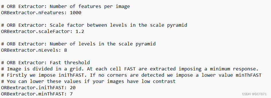
将nFeatures设置为2000
iniThFAST设置为10
minThFAST设置为3
四、在数据集中运行如下代码生成一个rgb文件用于slam
import numpy as np
import os
# 图片文件夹,后面的/不能省
from PIL import Image


img_path = 'D:/slam/phantom3-village-kfs-master/phantom3-village-kfs-master/'

# print(files)        # 当前路径下所有非目录子文件
# with open(img_path+"\opt_poses.txt") as f:
#     read_data = f.readlines()
# # print(read_data)
count = 0
for root, dirs, files in os.walk(img_path, topdown=False):
    print(root)     # 当前目录路径
    print(dirs)     # 当前目录下所有子目录
    with open("D:/slam/phantom3-village-kfs-master/phantom3-village-kfs-master"+"/rgb.txt", 'w') as g:
        # count = 0
        for i in files:
            # count = count +0.1
            # print(i[-3:-1]+i[-1])
            # if(i[-3:-1]+i[-1] == "jpg"):
            #     #print(count)
            #     #I = Image.open('./cadastre_gray/'+i)
            #     count = int(i[6:-1].split('.')[0])
            #     print(count)
            #     # print(read_data[count][0:7] +' '+ i)
            #     write_date[count] = time_list[count] +' '+ time_list[count]+'.jpg' +"\n"
            #     print(write_date[count])
            #     # print(read_data[count][0:7])
            #     #I.save('./picture/'+time_list[count]+'.jpg')

            # print(count)
            # print(i[0:9] + '.'+i[9] +i[11:17])
            #for i in range(10):
            #name = str(count)+".jpg"
            #g.writelines(str(count) + ' ' + name + '\n')
            print(i[0:-4])
            g.writelines(i[0:-4] + ' ' + i + '\n')
            # g.writelines(i[0:9] + '.'+i[9] +i[11:17]+ ' '+ i[0:9] + '.'+i[9] +i[11:17]+".jpg\n")
            #out.save('D:/slam/phantom3-village-kfs-master/phantom3-npu-master/phantom3-npu-master/npu/'+i)
            count = count + 0.01
        # for i in range(len(files)):
        #     print(write_date[i])
        #     # g.writelines(write_date[i])
        #     count=count+1
        # print(count)
# I = Image.open('./image.png')
# print(type(I))       #---><class 'PIL.JpegImagePlugin.JpegImageFile'>
# print(I.size)        #--->(1280, 720)
# I.show()
# I.save('./save.png')
随后将生成的KeyFrameTrajectory作为trajectory.txt运行map2dfusion的进程即可
其中将产生的点云文件用于ransac平面拟合,得到的结果用于config的plane中,即可得到相对优秀的融合结果。
ransac平面拟合如下
import random
import numpy as np
from math import acos, sin, cos, fabs, sqrt, log
from matplotlib import pyplot as plt
from mpl_toolkits.mplot3d import Axes3D
import csv
def new_csv():
    with open("pcltest.csv", "w") as csvfile:
        writer = csv.writer(csvfile)

        # 先写入columns_name
        # writer.writerow(["a", "b", "c", "d", "message"])
        writer.writerows([[1, 2, 3, 4, ',']])

def getData(filepath, row_need=1000):
    """
    加载数据并且取其中的部分行
    """
    data = np.loadtxt(filepath, delimiter=",")
    row_total = data.shape[0]
    print(row_total)
    row_sequence = np.arange(row_total)
    np.random.shuffle(row_sequence)

    return data[row_sequence[0:row_need], :]


def solve_plane(A, B, C):
    """
    求解平面方程
    :param A: 点A
    :param B: 点B
    :param C: 点C
    :return: Point(平面上一点),Quaternion(平面四元数),Nx(平面的法向量)
    """

    # 两个常量
    N = np.array([0, 0, 1])
    Pi = 3.1415926535

    # 计算平面的单位法向量,即BC 与 BA的叉积
    Nx = np.cross(B - C, B - A)
    Nx = Nx / np.linalg.norm(Nx)

    # 计算单位旋转向量与旋转角(范围为0到Pi)
    Nv = np.cross(Nx, N)
    angle = acos(np.dot(Nx, N))

    # 考虑到两个向量夹角不大于Pi/2,这里需要处理一下
    if angle > Pi / 2.0:
        angle = Pi - angle
        Nv = -Nv

    # FIXME: 此处如何确定平面上的一个点???
    # Point = (A + B + C) / 3.0
    Point = B
    # 计算单位四元数
    Quaternion = np.append(Nv * sin(angle / 2), cos(angle / 2))

    # print("旋转向量:\t", Nv)
    # print("旋转角度:\t", angle)
    # print("对应四元数:\t", Quaternion)

    return Point, Quaternion, Nx


def solve_distance(M, P, N):
    """
    求解点M到平面(P,Q)的距离
    :param M: 点M
    :param P: 平面上一点
    :param N: 平面的法向量
    :return: 点到平面的距离
    """

    # 从四元数到法向量
    # A = 2 * Q[0] * Q[2] + 2 * Q[1] * Q[3]
    # B = 2 * Q[1] * Q[2] - 2 * Q[0] * Q[3]
    # C = -Q[0] ** 2 - Q[1] ** 2 + Q[2] ** 2 + Q[3] ** 2
    # D = -A * P[0] - B * P[1] - C * P[2]

    # 为了计算简便,直接使用求解出的法向量
    A = N[0]
    B = N[1]
    C = N[2]
    D = -A * P[0] - B * P[1] - C * P[2]

    return fabs(A * M[0] + B * M[1] + C * M[2] + D) / sqrt(A ** 2 + B ** 2 + C ** 2)


def RANSAC(data):
    """
    使用RANSAC算法估算模型
    """
    # 数据规模
    SIZE = data.shape[0]
    # 迭代最大次数,每次得到更好的估计会优化iters的数值,默认10000
    iters = 10000
    # 数据和模型之间可接受的差值,默认0.25
    sigma = 0.15
    # 内点数目
    pretotal = 0
    # 希望的得到正确模型的概率,默认0.99
    Per = 0.999
    # 初始化一下
    P = np.array([])
    Q = np.array([])
    N = np.array([])
    for i in range(iters):
        # 随机在数据中选出三个点去求解模型
        sample_index = random.sample(range(SIZE), 3)
        P, Q, N = solve_plane(data[sample_index[0]], data[sample_index[1]], data[sample_index[2]])

        # 算出内点数目
        total_inlier = 0
        for index in range(SIZE):
            if solve_distance(data[index], P, N) < sigma:
                total_inlier = total_inlier + 1

        # 判断当前的模型是否比之前估算的模型好
        if total_inlier > pretotal:
            print(total_inlier / SIZE)
            iters = log(1 - Per) / log(1 - pow(abs(total_inlier / SIZE), 2))
            pretotal = total_inlier

        # 判断是否当前模型已经符合超过一半的点
        if total_inlier > SIZE / 2:
            break
    return P, Q, N


def draw(data, P, N):
    """
    画出散点图和平面
    :param data: 三维点
    :param N: 平面法向量
    """
    # 创建一个画布figure,然后在这个画布上加各种元素。
    fig = plt.figure()
    # 将画布作用于 Axes3D 对象上。
    ax = Axes3D(fig)

    # 画出散点图
    ax.scatter(data[0], data[1], data[2], c="gold")

    # 画出平面
    x = np.linspace(-30, 30, 10)
    y = np.linspace(-30, 30, 10)
    X, Y = np.meshgrid(x, y)
    Z = -(N[0] * X + N[1] * Y - (N[0] * P[0] + N[1] * P[1] + N[2] * P[2])) / N[2]
    ax.plot_surface(X, Y, Z)

    # 画出坐标轴
    ax.set_xlabel('X label')
    ax.set_ylabel('Y label')
    ax.set_zlabel('Z label')

    plt.show()


def test():
    A = np.random.randn(3)
    B = np.random.randn(3)
    C = np.random.randn(3)

    P, Q, N = solve_plane(A, B, C)
    print("Plane:\t", P, Q)

    D = np.random.randn(3)
    print("Point:\t", D)

    d = solve_distance(D, P, N)
    print("Distance:\t", d)


if __name__ == '__main__':
    data = getData("pcltest.csv")
    P, Q, N = RANSAC(data)
    print("Plane:\t", np.append(P, Q))
    draw(data.T, P, N)


 1601
1601


 被折叠的 条评论
为什么被折叠?
被折叠的 条评论
为什么被折叠?
 到【灌水乐园】发言


