机器学习每周挑战——客户流失数据预测

该篇文章探讨了通过分析客户数据,尤其是人口统计、金融行为和产品偏好等因素,预测客户流失的可能性。使用了LogisticRegression、DecisionTree、RandomForest和SVM等模型,并进行了特征重要性分析,以识别影响客户流失的关键驱动因素。
摘要由CSDN通过智能技术生成

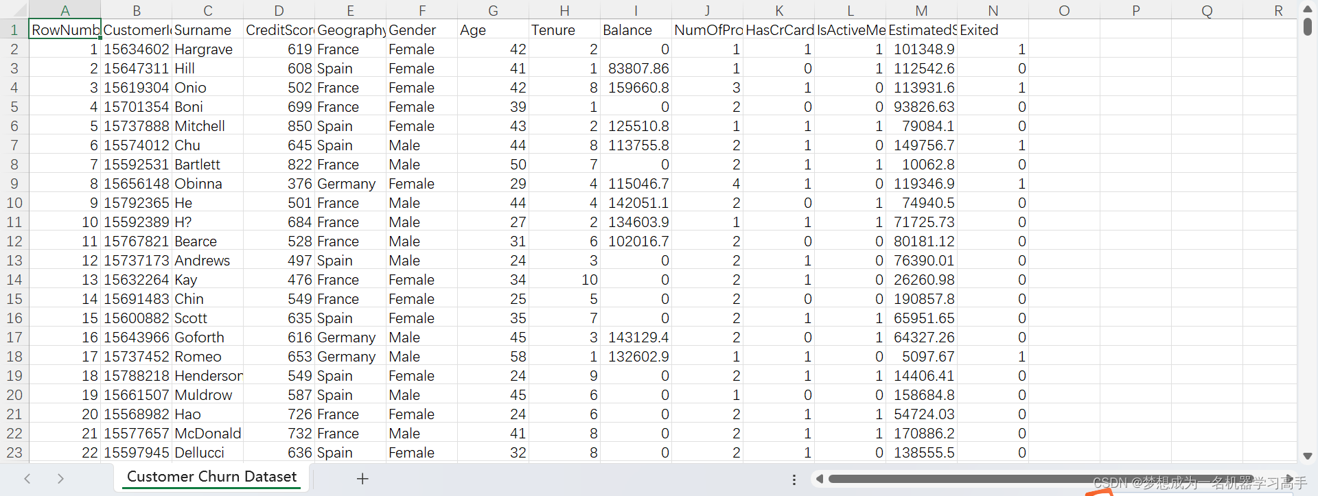
# 字段         说明
# RowNumber 每行数据的唯一标识符。
# CustomerId    客户的唯一标识符。
# Surname   客户的姓氏(出于隐私考虑,请对这些数据进行匿名处理)。
# CreditScore   客户在数据收集时的信用评分。
# Geography 客户所在的国家或地区,提供有关流失的地理趋势的见解。
# Gender    客户的性别。
# Age   客户的年龄,用于人口统计分析。
# Tenure    客户与银行合作的年限。
# Balance   客户的账户余额。
# NumOfProducts 客户购买或订阅的产品数量。
# HasCrCard 指示客户是否拥有信用卡(1表示是,0表示否)。
# IsActiveMember    指示客户是否为活跃会员(1表示是,0表示否)。
# EstimatedSalary   客户的预估工资。
# Exited    目标变量,指示客户是否已流失(1表示是,0表示否)。

import pandas as pd
import numpy as np
import matplotlib.pyplot as plt
import seaborn as sns
from sklearn.preprocessing import LabelEncoder,StandardScaler
from imblearn.over_sampling import SMOTE
from sklearn.model_selection import train_test_split
from sklearn.linear_model import LogisticRegression
from sklearn.tree import DecisionTreeClassifier
from sklearn.ensemble import RandomForestClassifier
from sklearn.svm import SVC
from sklearn.metrics import classification_report,confusion_matrix,accuracy_score
from hyperopt import fmin,tpe,hp
from hyperopt import STATUS_OK


data = pd.read_csv('Customer Churn Dataset.csv')
pd.set_option("display.max_row",1000)
pd.set_option("display.max_column",1000)

读入数据,同时导入需要用到的数据库对于数据的处理,我们可以发现前三列都是类似于ID的数据,对我们数据的分析没有任何用处,因此我们将前三列数据删除。

# 来看问题
# 探索性数据分析:通过多维度客户数据的深度挖掘,揭示潜在关联、趋势与异常,直观呈现客户特征与流失风险之间的内在关系。
# 客户细分:依据客户的人口统计特征、金融行为及产品偏好等信息,划分出具有不同流失倾向的群体,为精细化营销与服务策略提供依据。
# 流失预测建模:利用包含目标变量(Exited)的数据集训练预测模型,准确评估每个客户的未来流失概率,为预防性干预措施提供精准导向。
# 特征重要性分析:计算模型中各特征的贡献度或重要性得分,揭示影响客户流失的关键因素。
data_geography = pd.crosstab(data['Geography'],data['Exited'])
data_geography.plot(kind='bar',stacked=False,color=['blue','red'],figsize=(10,8))
plt.xlabel('地理因素')
plt.ylabel('客户流失数量')
plt.tight_layout()
# plt.show()

data_gender = pd.crosstab(data['Gender'],data['Exited'])
data_gender.plot(kind='bar',stacked=True,color=['green','pink'],figsize=(10,8))
plt.xlabel('性别因素')
plt.ylabel('客户流失数量')
plt.tight_layout()

bins = [0,20,30,40,50]
data['Age'] = pd.cut(data['Age'],bins=bins)
data_age = pd.crosstab(data['Age'],data['Exited'])
data_age.plot(kind='bar',stacked=True,color=['yellow','red'],figsize=(10,8))
plt.xlabel('年龄因素')
plt.ylabel('客户流失数量')
plt.tight_layout()

plt.show()


plt.figure(figsize=(10,8))
sns.boxplot(x=data['Exited'],y=data['Tenure'])
plt.xlabel('客户是否流失')
plt.xticks([0,1],labels=['已流失','未流失'])
plt.ylabel('与银行合作年限')
plt.tight_layout()


plt.figure(figsize=(10,8))
sns.boxplot(x=data['Exited'],y=data['Balance'])
plt.xlabel('客户是否流失')
plt.xticks([0,1],labels=['已流失','未流失'])
plt.ylabel('客户的银行账户余额')
plt.tight_layout()

plt.figure(figsize=(10,8))
sns.boxplot(x=data['Exited'],y=data['EstimatedSalary'],
            medianprops={'color':'green'},flierprops={'markerfacecolor':'blue','markeredgecolor':'red'},
            #  指定中值线的颜色,为绿色           指定离群点的填充颜色和离群点的边框颜色(边框颜色不经常用)
            boxprops={'facecolor':'yellow'})
            # 指定箱型图内的颜色
plt.xlabel('客户是否流失')
plt.xticks([0,1],labels=['已流失','未流失'])
plt.ylabel('客户的预估工资')
plt.tight_layout()
# 由于设置箱型图颜色较为复杂,因此我只在一个箱型图中进行设置,
# plt.show()


data_numproduct = data['NumOfProducts'].value_counts().reset_index()
plt.figure(figsize=(10,8))
plt.pie(data_numproduct['count'],labels=data_numproduct['NumOfProducts'],autopct='%1.1f%%')
plt.title('购买产品数量与客户流失之间的关系')


data_hascard = data['HasCrCard'].value_counts().reset_index()
plt.figure(figsize=(10,8))
plt.pie(data_hascard['count'],labels=data_hascard['HasCrCard'].map({0:'未拥有',1:'拥有'}),autopct='%1.1f%%')
plt.title('是否有信用卡与客户流失之间的关系')


data_activemenber = data['IsActiveMember'].value_counts().reset_index()
plt.figure(figsize=(10,8))
plt.pie(data_activemenber['count'],labels=data_activemenber['IsActiveMember'].map({0:'不是活跃会员',1:'是活跃会员'}),autopct='%1.1f%%')
plt.title('客户是否活跃与客户流失之间的关系')

plt.show()


 最后我们对数据进行建模

le = LabelEncoder()
for col in data.columns[:-1]:
    data[col] = le.fit_transform(data[col])

# 将分类数据转换为数值型数据后,我们可以发现部分数据跨度非常大,从0到几万,而部分数据只有0,1。因此我们必须对数据进行标准化,
# 即将数据缩放到相同的区间内
# scaler = StandardScaler()
# data_feature = data.iloc[:,0:10]
# data_feature = scaler.fit_transform(data_feature)

log = LogisticRegression(max_iter=10000)
Dtree = DecisionTreeClassifier()
Rtree = RandomForestClassifier()


models = [log,Dtree,Rtree]
# X = data_feature
X = data.iloc[:,:-1]
y = data.iloc[:,-1]
X_train,X_test,y_train,y_test = train_test_split(X,y,test_size=0.3,random_state=42)
# 由于数据存在不均衡现象,因此我们对数据进行重采样
# X_smote,y_smote = SMOTE().fit_resample(X_train,y_train)
# X_smote = scaler.fit_transform(X_smote)

for model in models:
    model.fit(X_train,y_train)
    y_pred = model.predict(X_test)
    class_report = classification_report(y_test,y_pred)
    print(model.__class__.__name__)
    print(class_report)

    # 模型的混淆矩阵
    corr = confusion_matrix(y_test,y_pred)
    plt.figure(figsize=(10,8))
    sns.heatmap(corr,cmap='viridis',annot=True,fmt='.2f')
    plt.title(model.__class__.__name__+'的混淆矩阵')

plt.show()

importance = Rtree.feature_importances_
sort_importance = importance.argsort()
feature = X.columns

plt.figure()
plt.barh(range(len(sort_importance)),importance[sort_importance])
plt.yticks(range(len(sort_importance)), [feature[i] for i in sort_importance])
plt.title('特征重要性分析')
plt.xlabel("特征重要性")
plt.show()

LogisticRegression
              precision    recall  f1-score   support

           0       0.83      0.97      0.89      2416
           1       0.59      0.16      0.26       584

    accuracy                           0.82      3000
   macro avg       0.71      0.57      0.57      3000
weighted avg       0.78      0.82      0.77      3000

DecisionTreeClassifier
              precision    recall  f1-score   support

           0       0.88      0.87      0.87      2416
           1       0.47      0.50      0.48       584

    accuracy                           0.79      3000
   macro avg       0.67      0.68      0.68      3000
weighted avg       0.80      0.79      0.80      3000

RandomForestClassifier
              precision    recall  f1-score   support

           0       0.88      0.96      0.92      2416
           1       0.76      0.46      0.57       584

    accuracy                           0.87      3000
   macro avg       0.82      0.71      0.74      3000
weighted avg       0.86      0.87      0.85      3000

SVC
              precision    recall  f1-score   support

           0       0.86      0.98      0.92      2416
           1       0.83      0.36      0.50       584

    accuracy                           0.86      3000
   macro avg       0.85      0.67      0.71      3000
weighted avg       0.86      0.86      0.84      3000


  • 17
    点赞
  • 9
    收藏
    觉得还不错? 一键收藏
  • 0
    评论
评论
添加红包

请填写红包祝福语或标题

红包个数最小为10个

红包金额最低5元

当前余额3.43前往充值 >
需支付:10.00
成就一亿技术人!
领取后你会自动成为博主和红包主的粉丝 规则
hope_wisdom
发出的红包
实付
使用余额支付
点击重新获取
扫码支付
钱包余额 0

抵扣说明:

1.余额是钱包充值的虚拟货币,按照1:1的比例进行支付金额的抵扣。
2.余额无法直接购买下载,可以购买VIP、付费专栏及课程。

余额充值