


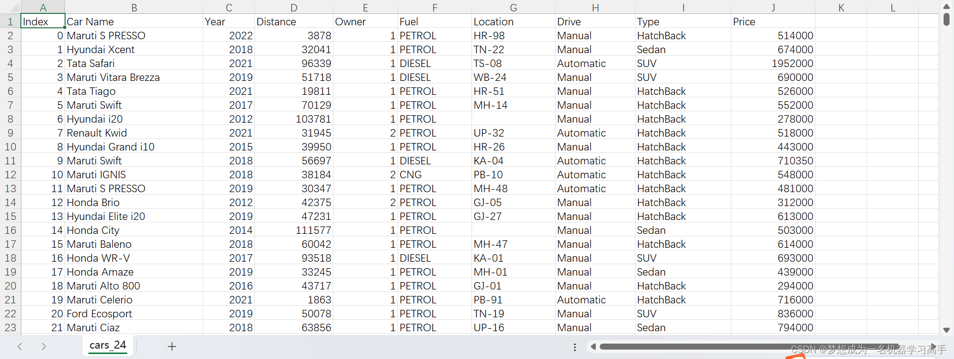
这是数据集的截图
目录
背景描述
本数据爬取自印度最大的二手车交易平台 CARS24,包含 8000+ 该平台上交易车辆的关键评估信息。
CARS24 成立于 2015 年,总部位于印度古尔冈,是一个在印度、澳大利亚、泰国和阿联酋运营的二手车交易平台,为用户提供一站式二手车交易服务,包括车辆评估、交易、融资、保险等。CARS24 已成为印度最大的二手车交易平台之一,在印度拥有超过 1000 家线下门店。
数据说明
| 字段 | 说明 |
|---|---|
| Car Name | 汽车品牌或汽车型号 |
| Distance | 行驶里程 (单位:公里) |
| Year Bought | 购车年份 |
| Previous Owners | 前任车主数量 |
| Location | 车管所所在地 |
| Transmission | 变速箱类型 (automatic自动 或 manua手动) |
| Car Type | 车型 |
| Fuel | 燃料类型 (汽油、柴油、CNG 等) |
| Price | 价格 |
-
车型对照:
英文 中文 sedan 轿车 SUV SUV hatchback 两厢车 luxury SUV 豪华SUV luxury sedan 豪华轿车 -
燃料类型对照:
英文 中文 petrol 汽油 diesel 柴油 CNG 压缩天然气 other 其他
老规矩,第一步先导入用到的库
import pandas as pd
import numpy as np
import seaborn as sns
import matplotlib.pyplot as plt
from sklearn.metrics import confusion_matrix
import statsmodels.api as sm
from statsmodels.formula.api import ols
from sklearn.preprocessing import StandardScaler,LabelEncoder,OneHotEncoder
from statsmodels.stats.outliers_influence import variance_inflation_factor
from sklearn.model_selection import train_test_split,cross_val_score
from sklearn.linear_model import LinearRegression
from sklearn.metrics import mean_squared_error,r2_score,classification_report
import scipy.stats as stats
from statsmodels.stats.stattools import durbin_watson
from statsmodels.stats.diagnostic import het_breuschpagan
from scipy.stats import kstest
from sklearn.ensemble import RandomForestRegressor
from hyperopt import fmin, tpe, hp,STATUS_OK
第二步,读入数据:
data = pd.read_csv('cars_24.csv')
pd.set_option('display.max_columns',1000)
pd.set_option('display.max_rows',1000)

plt.rcParams['axes.unicode_minus'] = False
plt.rcParams['font.family'] = ['Microsoft YaHei']
第三步,数据预处理
print(data.info()) # 从这里我们可以看出Location Year Car Name 三列数据有确实值,由于位置信息无法填充,因此我选择将缺失值删除
data.dropna(inplace=True)
for col in data.columns:
    print(col)
    print(data[col].unique())
    print('/'*20)
# 通过上面的循环我们可以了解到所有列的唯一值,排除Index Distance Price这些连续值,我们可以看出其他特征列都有那些值
# 删除包含22-BH的行,因为在印度的车辆注册号码中,BH通常不是一个标准的州或联邦领地代码,这可能是数据有误,这里直接删除
data = data[data['Location'] != '22-BH']
# 由于Car Name名字太多,因此我们只提取品牌,即,第一个空格前面的
data['Brand'] = data['Car Name'].apply(lambda x: x.split()[0])
# 有了Brand后,我们将原先的Car Name这一列删除
data = data.drop('Car Name',axis=1)
data['Location'] = data['Location'].apply(lambda x:x[:2])
# print(data['Location'].unique())           # 如果前面我们没发现22-BH这种异常值,我们从这里发现后,我们也可以将其删除
# data['Location'] = [x for x in data['Location'] if x!=22]
# 标签这一列对于我们来说也没有用,因此我们也将其删除
data.drop('Index',axis=1,inplace=True)
# 将年份转换为整数
data['Year'] = data['Year'].astype(int)
# 我们对预处理后的数据进行复制,以便于我们后续对数据进行建模
new_data = data.copy()
第四步:对数据的分析
# 接下来我们对数据进行分析,通过图表来观察他们各个特征之间的关联
plt.figure(figsize=(10,8))
ax = sns.countplot(x='Brand',data=data)
plt.title('不同品牌的分布情况')
plt.xlabel('品牌')
plt.ylabel('品牌数量')
plt.xticks(rotation=90)
plt.tight_layout()

for p in ax.patches:
    ax.annotate(format(p.get_height(), '.0f'),
                (p.get_x() + p.get_width() / 2., p.get_height()),
                ha = 'center', va = 'center',
                xytext = (0, 10),
                textcoords = 'offset points')

plt.show()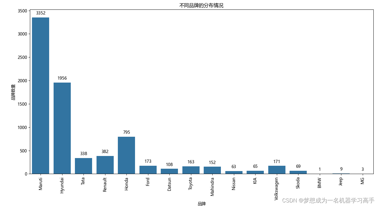
所有二手车品牌中,马鲁蒂(Maruti)和现代(Hyundai)的数量是最多的,马鲁蒂是印度的一个知名品牌,所以占比也是最大的
fig,ax = plt.subplots(1,3,figsize=(10,8))
count_year = data['Year'].value_counts()
label = count_year.index
# print(label)
ax[0].pie(count_year,labels=label,autopct='%.2f%%')
ax[0].set_title('各个年份购车数量占比')

ax[1].hist(data['Distance'],bins=30)
ax[1].set_title('车辆行驶距离')

ax[2].hist(data['Price'],bins=30)
ax[2].set_title('购车价格')

plt.tight_layout()
plt.show()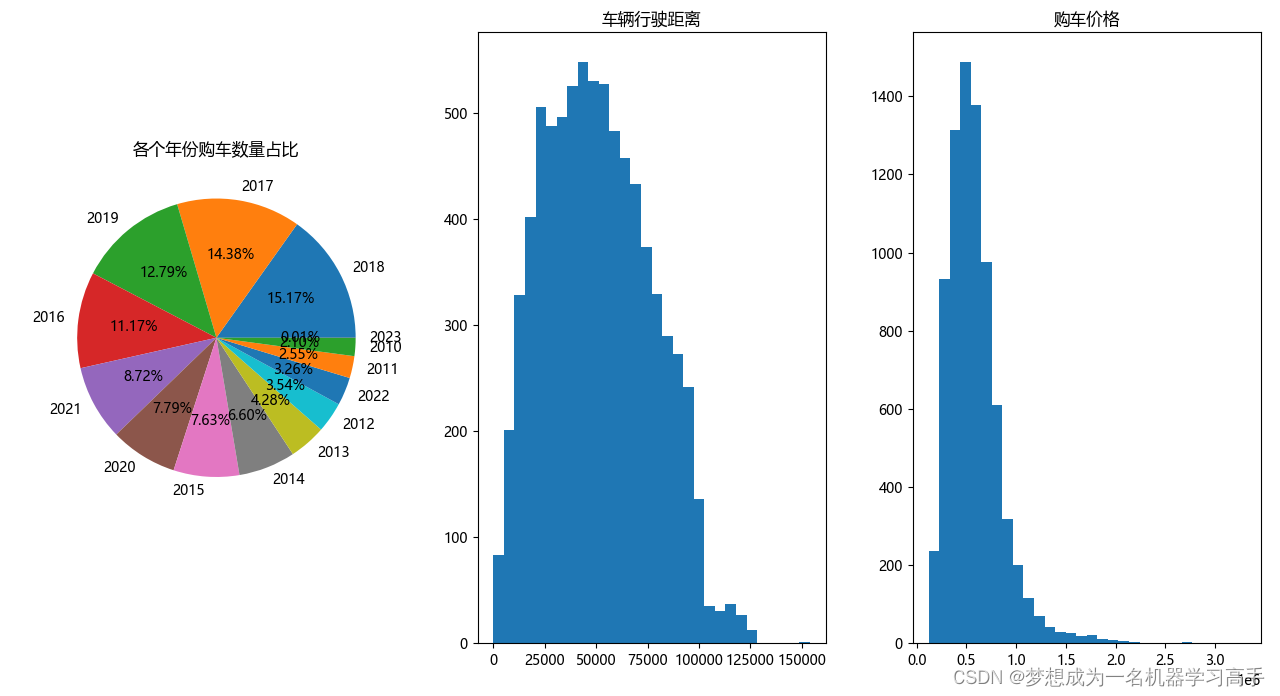
总结:数据集中的车辆大多数是17,18年购买的,有较短的行驶距离,且价格相对较低
fig,ax = plt.subplots(2,2,figsize=(10,8))
owner_plot = sns.countplot(ax=ax[0,0],x='Owner',data=data)
ax[0,0].set_title('前任车主特征分布图')
ax[0,0].set_xlabel('前任车主')
ax[0,0].set_ylabel('总数')
for x in owner_plot.patches:
    owner_plot.annotate(format(x.get_height(),'.0f'),
                        (x.get_x()+x.get_width()/2,x.get_height()),
                        ha='center',va='center',
                        xytext=(0,10),
                        textcoords='offset points')


fuel_plot = sns.countplot(ax=ax[0,1],x='Fuel',data=data)
ax[0,1].set_title('燃料类型特征分布图')
ax[0,1].set_xlabel('燃料类型')
ax[0,1].set_ylabel('总数')
for x in fuel_plot.patches:
    fuel_plot.annotate(format(x.get_height(),'.0f'),
                        (x.get_x()+x.get_width()/2,x.get_height()),
                        ha='center',va='center',
                        xytext=(0,10),
                        textcoords='offset points')


drive_plot = sns.countplot(ax=ax[1,0],x='Drive',data=data)
ax[1,0].set_title('变速器类型特征分布图')
ax[1,0].set_xlabel('变速器类型')
ax[1,0].set_ylabel('总数')
for x in drive_plot.patches:
    drive_plot.annotate(format(x.get_height(),'.0f'),
                        (x.get_x()+x.get_width()/2,x.get_height()),
                        ha='center',va='center',
                        xytext=(0,10),
                        textcoords='offset points')


type_plot = sns.countplot(ax=ax[1,1],x='Type',data=data)
ax[1,1].set_title('车辆类型特征分布图')
ax[1,1].set_xlabel('车辆类型')
ax[1,1].set_ylabel('总数')
for x in type_plot.patches:
    type_plot.annotate(format(x.get_height(),'.0f'),
                        (x.get_x()+x.get_width()/2,x.get_height()),
                        ha='center',va='center',
                        xytext=(0,10),
                        textcoords='offset points')
plt.tight_layout()
plt.show() 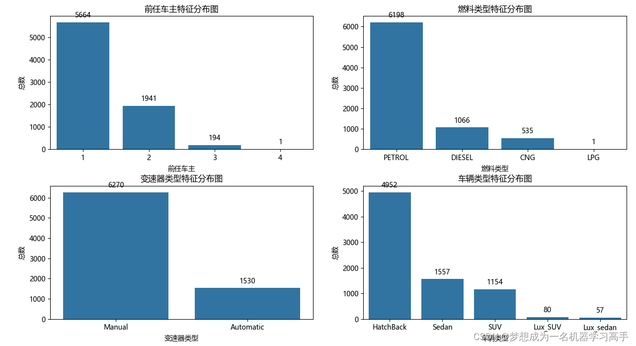
1.大多数车都是一手车(只有一个前任车主)。
2.大多数车都是使用汽油(Petrol),然后就是柴油(Diesel),天然气(CNG)和液化石油气(LPG)作为燃料类型的车辆数量相对较少。
3.手动挡(Manual)车辆数量大于自动挡(Automatic)车辆数量。
4.掀背车(HatchBack)是最常见的车型,其次是轿车(Sedan)和SUV,豪华SUV(Lux_SUV)和豪华轿车(Lux_sedan)的数量相对较少。
plt.figure(figsize=(10,8))
registration = data['Location'].value_counts().reset_index()
# print(registration)
plt.bar(registration['Location'],registration['count'])
plt.title('车辆注册地址')
plt.xlabel('注册地')
plt.ylabel('数量')
plt.tight_layout()
plt.show()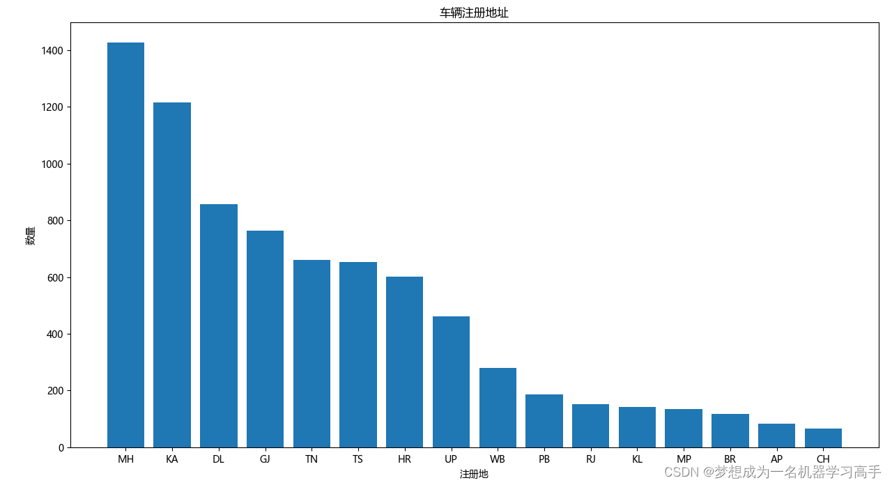
MH和KA有较多的车辆注册,CH、KL、RJ、BR、AP、MP有较少的车辆注册,较少的注册数量可能表明在某些州二手车市场的规模较小。
plt.figure(figsize=(10,8))
sns.boxplot(x='Brand',y='Price',data=data)
plt.title('品牌和价格分布的箱线图')
plt.xlabel('品牌')
plt.ylabel('价格')
plt.tight_layout()
plt.show()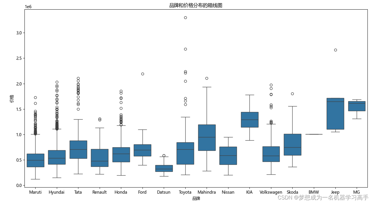
 最低0.47元/天 解锁文章


 4万+
4万+

 被折叠的 条评论
为什么被折叠?
被折叠的 条评论
为什么被折叠?
 到【灌水乐园】发言


