深度学习训练营之天气识别P3

最新推荐文章于 2024-05-31 16:14:40 发布

无你想你

最新推荐文章于 2024-05-31 16:14:40 发布

阅读量353

点赞数

分类专栏：深度学习文章标签：深度学习 tensorflow python

本文链接：https://blog.csdn.net/qq_62904883/article/details/128292778

版权

深度学习专栏收录该内容

27 篇文章 1 订阅

订阅专栏

深度学习训练营之天气识别

原文链接
环境介绍
前置工作
数据预处理
构建CNN网络
编译
模型训练
结果可视化

原文链接

🍨 本文为🔗365天深度学习训练营中的学习记录博客
🍦 参考文章：365天深度学习训练营-第P3周：天气识别
🍖 原作者：K同学啊|接辅导、项目定制

环境介绍

语言环境：Python3.9.13
编译器：jupyter notebook
深度学习环境：TensorFlow2

前置工作

设置GPU

如果使用的是CPU就不用设置了

import tensorflow as tf

gpus = tf.config.list_physical_devices("GPU")

if gpus:
    gpu0 = gpus[0]                                        #如果有多个GPU，仅使用第0个GPU
    tf.config.experimental.set_memory_growth(gpu0, True)  #设置GPU显存用量按需使用
    tf.config.set_visible_devices([gpu0],"GPU")

导入数据

对数据进行导入,首先是导入需要的包

import matplotlib.pyplot as plt
import os,PIL

# 设置随机种子尽可能使结果可以重现
import numpy as np
np.random.seed(1)

# 设置随机种子尽可能使结果可以重现
import tensorflow as tf
tf.random.set_seed(1)

from tensorflow import keras
from tensorflow.keras import layers,models

import pathlib

调整数据集所在的位置
在这里插入图片描述

data_dir = "D:/BaiduNetdiskDownload/fiveday/fiveday-3/weather_photos/"
data_dir = pathlib.Path(data_dir)

数据查看

数据集一共分为cloudy、rain、shine、sunrise四类，分别存放于weather_photos文件夹中以各自名字命名的子文件夹中。

image_count = len(list(data_dir.glob('*/*.jpg')))
print("图片总数为：",image_count)

图片总数为： 1125

roses = list(data_dir.glob('sunrise/*.jpg'))
PIL.Image.open(str(roses[3]))

在这里插入图片描述

数据预处理

加载数据

使用image_dataset_from_directory方法将磁盘中的数据加载到tf.data.Dataset中

batch_size = 32
img_height = 180
img_width = 180

"""
关于image_dataset_from_directory()的详细介绍可以参考文章：https://mtyjkh.blog.csdn.net/article/details/117018789
"""
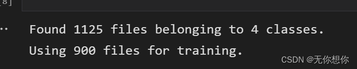
train_ds = tf.keras.preprocessing.image_dataset_from_directory(
    data_dir,
    validation_split=0.2,
    subset="training",
    seed=123,
    image_size=(img_height, img_width),
    batch_size=batch_size)

在这里插入图片描述
通过class_names输出数据集的标签,标签按照字母顺序对应于目录名称

class_names = train_ds.class_names
print(class_names)

在这里插入图片描述

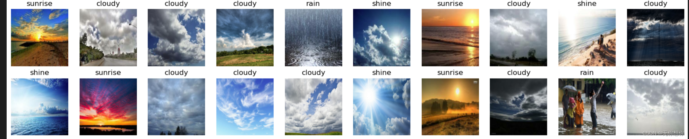
可视化数据

plt.figure(figsize=(20, 10))

for images, labels in train_ds.take(1):
    for i in range(20):
        ax = plt.subplot(5, 10, i + 1)

        plt.imshow(images[i].numpy().astype("uint8"))
        plt.title(class_names[labels[i]])
        
        plt.axis("off")

在这里插入图片描述

检查数据

for image_batch, labels_batch in train_ds:
    print(image_batch.shape)
    print(labels_batch.shape)
    break

在这里插入图片描述

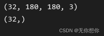
Image_batch是形状的张量（32,180,180,3）。这是一批形状180x180x3的32张图片（最后一维指的是彩色通道RGB）。
Label_batch是形状（32，）的张量，这些标签对应32张图片

配置数据集

shuffle()：打乱数据，关于此函数的详细介绍可以参考：https://zhuanlan.zhihu.com/p/42417456
prefetch()：预取数据，加速运行

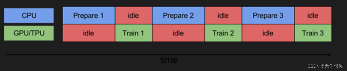
`prefetch()`功能详细介绍：

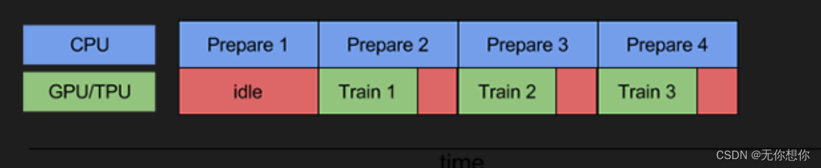
CPU 正在准备数据时，加速器处于空闲状态。相反，当加速器正在训练模型时，CPU 处于空闲状态。因此，训练所用的时间是 CPU 预处理时间和加速器训练时间的总和。prefetch()将训练步骤的预处理和模型执行过程重叠到一起。当加速器正在执行第 N 个训练步时，CPU 正在准备第 N+1 步的数据。这样做不仅可以最大限度地缩短训练的单步用时（而不是总用时），而且可以缩短提取和转换数据所需的时间。如果不使用prefetch()，CPU 和 GPU/TPU 在大部分时间都处于空闲状态
使用该函数的作用就在于尽可能的提高CPU等的使用性能,提高模型训练时候的速度
在这里插入图片描述
使用该函数可以减少空闲时间

cache():将数据集缓存到内存当中,加速运行

AUTOTUNE = tf.data.AUTOTUNE

train_ds = train_ds.cache().shuffle(1000).prefetch(buffer_size=AUTOTUNE)
val_ds = val_ds.cache().prefetch(buffer_size=AUTOTUNE)

构建CNN网络

卷积神经网络（CNN）的输入是张量 (Tensor) 形式的 (image_height, image_width, color_channels)，包含了图像高度、宽度及颜色信息。不需要输入batch size。color_channels 为 (R,G,B) 分别对应 RGB 的三个颜色通道（color channel）。在此示例中，我们的 CNN 输入，fashion_mnist 数据集中的图片，形状是 (28, 28, 1)即灰度图像。我们需要在声明第一层时将形状赋值给参数input_shape。

num_classes = 5

"""
关于卷积核的计算不懂的可以参考文章：https://blog.csdn.net/qq_38251616/article/details/114278995

layers.Dropout(0.4) 作用是防止过拟合，提高模型的泛化能力。
在上一篇文章花朵识别中，训练准确率与验证准确率相差巨大就是由于模型过拟合导致的

关于Dropout层的更多介绍可以参考文章：https://mtyjkh.blog.csdn.net/article/details/115826689
"""

model = models.Sequential([
    layers.experimental.preprocessing.Rescaling(1./255, input_shape=(img_height, img_width, 3)),
    
    layers.Conv2D(16, (3, 3), activation='relu', input_shape=(img_height, img_width, 3)), # 卷积层1，卷积核3*3  
    layers.AveragePooling2D((2, 2)),               # 池化层1，2*2采样
    layers.Conv2D(32, (3, 3), activation='relu'),  # 卷积层2，卷积核3*3
    layers.AveragePooling2D((2, 2)),               # 池化层2，2*2采样
    layers.Conv2D(64, (3, 3), activation='relu'),  # 卷积层3，卷积核3*3
    layers.Dropout(0.3),  
    
    layers.Flatten(),                       # Flatten层，连接卷积层与全连接层
    layers.Dense(128, activation='relu'),   # 全连接层，特征进一步提取
    layers.Dense(num_classes)               # 输出层，输出预期结果
])

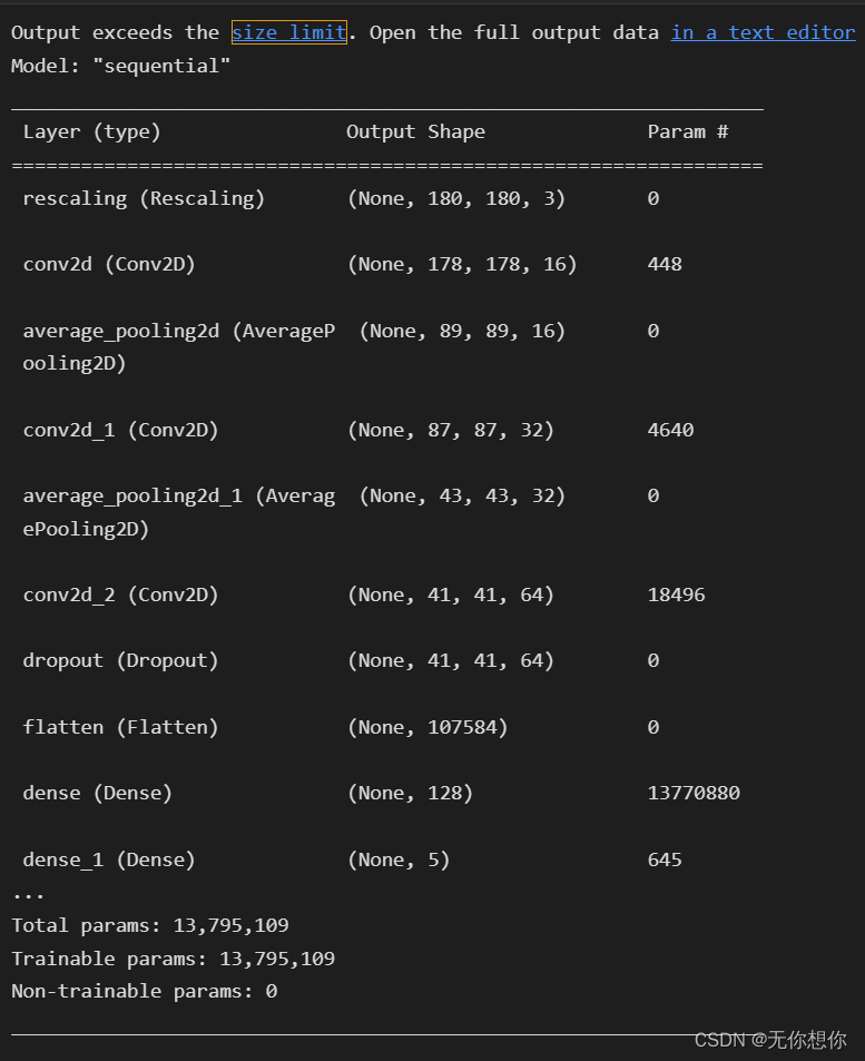
model.summary()  # 打印网络结构

在这里插入图片描述

编译

在准备对模型进行训练之前，还需要再对其进行一些设置。以下内容是在模型的编译步骤中添加的：

损失函数（loss）：用于衡量模型在训练期间的准确率。
优化器（optimizer）：决定模型如何根据其看到的数据和自身的损失函数进行更新。
指标（metrics）：用于监控训练和测试步骤。以下示例使用了准确率，即被正确分类的图像的比率。

# 设置优化器
opt = tf.keras.optimizers.Adam(learning_rate=0.001)

model.compile(optimizer=opt,
              loss=tf.keras.losses.SparseCategoricalCrossentropy(from_logits=True),
              metrics=['accuracy'])

模型训练

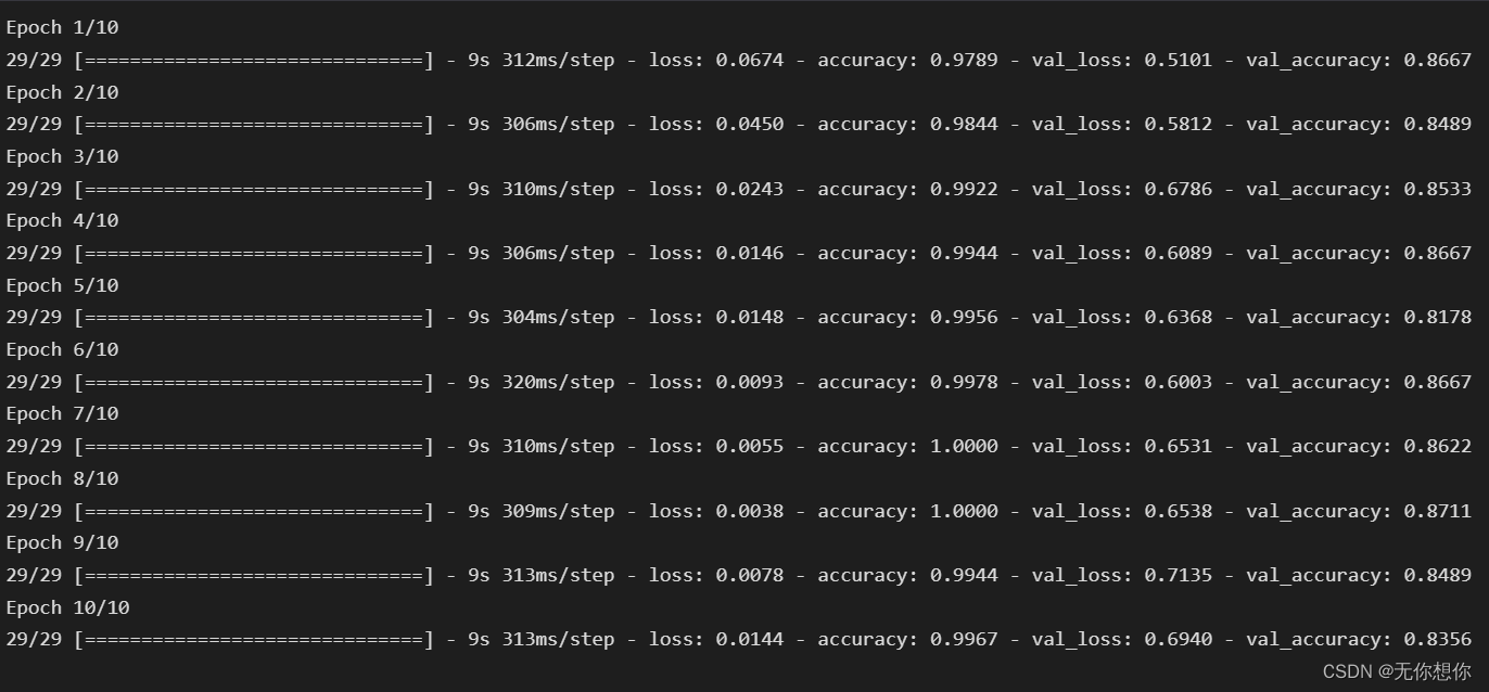
epochs = 10

history = model.fit(
  train_ds,
  validation_data=val_ds,
  epochs=epochs
)

在这里插入图片描述

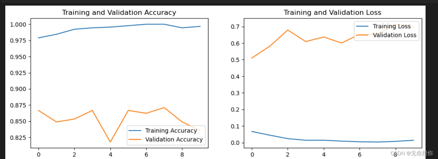
结果可视化

对模型进行评估

acc = history.history['accuracy']
val_acc = history.history['val_accuracy']

loss = history.history['loss']
val_loss = history.history['val_loss']

epochs_range = range(epochs)

plt.figure(figsize=(12, 4))
plt.subplot(1, 2, 1)
plt.plot(epochs_range, acc, label='Training Accuracy')
plt.plot(epochs_range, val_acc, label='Validation Accuracy')
plt.legend(loc='lower right')
plt.title('Training and Validation Accuracy')

plt.subplot(1, 2, 2)
plt.plot(epochs_range, loss, label='Training Loss')
plt.plot(epochs_range, val_loss, label='Validation Loss')
plt.legend(loc='upper right')
plt.title('Training and Validation Loss')
plt.show()