在MNIST上用Pytorch跑跑GPU

目录

前言

一、Pytorch的入门

二、使用步骤

1.引入库

2.读入数据

3.定义卷积神经网络

4.Training

5.在测试集上测试模型

总结

---

前言

深度学习中有很多入门数据，MNIST被称为机器学习的“Hello World”，一个人能否入门深度学习往往就是以能否玩转MNIST数据来判断的。

PyTorch有一个很好的模块nn，它提供了一种有效构建大型神经网络的好方法。

我们将按顺序执行以下步骤：

1. 使用torchvision加载并标准化 MNIST 训练和测试数据集
2. 定义卷积神经网络
3. 根据训练数据训练网络
4. 在测试数据上测试网络

---

提示：以下是本篇文章正文内容，下面案例可供参考

一、Pytorch的入门

安装命令
https://pytorch.org/
官方文档
https://pytorch.org/tutorials/beginner/blitz/tensor_tutorial.html

中文文档
https://pytorch.apachecn.org/docs/1.7/03.html
 

二、使用步骤

1.引入库

代码如下（示例）：

import torch
import torch.nn as nn
import torch.nn.functional as F
import torch.optim as optim
import torchvision
import torchvision.transforms as transforms

TorchVision 数据集的输出是[0, 1]范围的PILImage图像。 我们将它们转换为归一化范围[-1, 1]的张量。 .. 注意：

If running on Windows and you get a BrokenPipeError, try setting
the num_worker of torch.utils.data.DataLoader() to 0.

 

2.读入数据

代码如下（示例）：

#一些参数
batch_size_train = 200
batch_size_test = 1000
learning_rate = 0.0073564225
momentum = 0.9
random_seed = 1
torch.manual_seed(random_seed)

transform = transforms.Compose(
    [transforms.ToTensor(),# PIL Image → Tensor
    transforms.Normalize((0.1307,),(0.3081,))]  # 0,1 →  -1,1
)

trainset = torchvision.datasets.MNIST(download=True,root='./data',train=True,transform=transform)
trainloader = torch.utils.data.DataLoader(trainset,batch_size=batch_size_train,shuffle=True,num_workers=2)
testset = torchvision.datasets.MNIST(download=True,root='./data',train=False,transform=transform)
testloader = torch.utils.data.DataLoader(testset,batch_size=batch_size_test,shuffle=True,num_workers=2)

# explore testing data
examples = enumerate(trainloader)
batch_idx, (example_data, example_targets) = next(examples)
print(example_targets)
print(example_data.shape)

tensor([4, 4, 2, 2, 5, 4, 4, 5, 4, 4, 7, 6, 6, 9, 5, 9, 1, 3, 1, 8, 8, 1, 6, 9,
        0, 5, 4, 9, 7, 3, 2, 4, 2, 2, 7, 1, 8, 2, 2, 8, 9, 9, 2, 4, 6, 9, 1, 8,
        2, 7, 3, 0, 7, 8, 4, 7, 0, 7, 8, 3, 6, 1, 0, 3, 6, 5, 4, 2, 1, 1, 0, 4,
        5, 2, 6, 5, 6, 4, 9, 1, 8, 2, 6, 7, 5, 6, 6, 6, 0, 8, 3, 3, 9, 6, 1, 7,
        2, 4, 1, 1, 8, 4, 1, 9, 2, 7, 7, 1, 2, 1, 2, 4, 2, 5, 7, 9, 5, 7, 5, 7,
        7, 6, 7, 2, 9, 5, 3, 4, 1, 1, 2, 7, 4, 5, 3, 0, 4, 9, 9, 3, 4, 3, 0, 6,
        7, 0, 7, 4, 1, 7, 5, 3, 6, 5, 7, 1, 0, 6, 8, 3, 5, 5, 2, 6, 1, 7, 2, 3,
        2, 1, 4, 9, 6, 4, 4, 0, 9, 1, 9, 7, 9, 9, 5, 9, 7, 2, 0, 5, 6, 1, 4, 5,
        7, 3, 3, 9, 5, 5, 6, 5])
torch.Size([200, 1, 28, 28])

example_data.shape

torch.Size([200, 1, 28, 28])

展示数据（示例）：

import matplotlib.pyplot as plt
fig = plt.figure()
for i in range(6):
  plt.subplot(2,3,i+1)
  plt.tight_layout()
  plt.imshow(example_data[i][0], cmap='gray', interpolation='none')
  plt.title("Ground Truth: {}".format(example_targets[i]))
  plt.xticks([])
  plt.yticks([])
plt.show()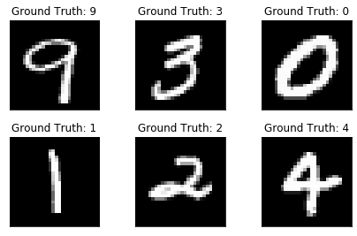

3.定义卷积神经网络

# 卷积神经网络
class Net(nn.Module):
    def __init__(self):
        super(Net,self).__init__()
        self.conv1 = nn.Conv2d(1,6,5)
        self.pool = nn.MaxPool2d(2,2)
        self.conv2 = nn.Conv2d(6,16,3)
        self.fc1 = nn.Linear(16*5*5,120) #3-dim (0,1,2)
        self.fc2 = nn.Linear(120,84)
        self.fc3 = nn.Linear(84,10)
    def forward(self,x):
        x = self.pool(F.relu(self.conv1(x)))
        x = self.pool(F.relu(self.conv2(x)))#
        #print(x.size()) # 4*16*5*5
        x = x.view(-1,16*5*5)
        x = F.relu(self.fc1(x))
        x = F.relu(self.fc2(x))
        x = self.fc3(x)
        return x
net = Net()

对数字图像进行分类的网络：

因为MNIST本来就是28*28的尺寸，所以把此处两个5*5的filter,改为第一个5*5，第二个3*3

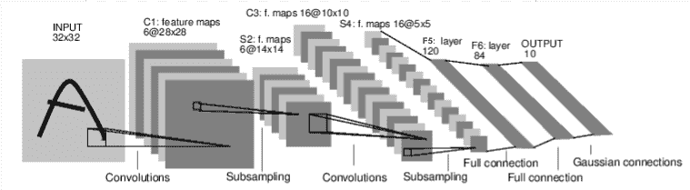
input -> conv2d(5*5) -> relu -> maxpool2d(2*2,stride=2) -> conv2d(3*3) -> relu -> maxpool2d
      -> view -> linear -> relu -> linear -> relu -> linear
      -> CrossEntropyLoss
      -> loss.backward()

GPU（示例）：

device = torch.device("cuda:0" if torch.cuda.is_available() else "cpu")
net = net.to(device)

优化设置（示例）：

optimizer = optim.SGD(net.parameters(),lr=learning_rate,momentum=momentum)
# 损失函数
criterion = nn.CrossEntropyLoss()

 

4.Training

# 训练
for epoch in range(10):
    running_loss = 0.0
    for i,data in enumerate(trainloader,0):
        images,labels = data
        images = images.to(device)
        labels = labels.to(device)
        optimizer.zero_grad()
        outputs = net(images).to(device)
        loss = criterion(outputs,labels)
        loss.backward()
        optimizer.step()
        running_loss += loss.item()
        if i%200 == 199:
            print(f'{epoch+1}, {i+1}; loss:{running_loss/200}')
            running_loss = 0.0
print('Finished Traing')

[epoch:1] Train_Acc:0.11535599820315834
[epoch:2] Train_Acc:0.8604069556295871
[epoch:3] Train_Acc:0.9161073217416803
[epoch:4] Train_Acc:0.9347538277755181
[epoch:5] Train_Acc:0.9468421627922604
[epoch:6] Train_Acc:0.9534654732731481
[epoch:7] Train_Acc:0.9601991592611496
[epoch:8] Train_Acc:0.9640288649282108
[epoch:9] Train_Acc:0.9678141941968351
[epoch:10] Train_Acc:0.9717304096945251
[epoch:11] Train_Acc:0.9740558569591182
[epoch:12] Train_Acc:0.9762585523794405
[epoch:13] Train_Acc:0.9784671182620028
[epoch:14] Train_Acc:0.980622759067531
[epoch:15] Train_Acc:0.9825073758035433
[epoch:16] Train_Acc:0.9835698009208621
[epoch:17] Train_Acc:0.9849561475085405
[epoch:18] Train_Acc:0.984593168948583
[epoch:19] Train_Acc:0.9861344359718108
[epoch:20] Train_Acc:0.9884813274582848
......
[epoch:81] Train_Acc:0.9999008766757591
[epoch:82] Train_Acc:0.9999041514335644
[epoch:83] Train_Acc:0.9999067126787554
[epoch:84] Train_Acc:0.9999060793153816
[epoch:85] Train_Acc:0.999907713802285
[epoch:86] Train_Acc:0.9999101123808362
[epoch:87] Train_Acc:0.999913753370562
[epoch:88] Train_Acc:0.9999169482896999
[epoch:89] Train_Acc:0.9999179632678806
[epoch:90] Train_Acc:0.9999185223209414
[epoch:91] Train_Acc:0.9999210347178238
[epoch:92] Train_Acc:0.999922851408459
[epoch:93] Train_Acc:0.9999243181449081
[epoch:94] Train_Acc:0.999926438184635
[epoch:95] Train_Acc:0.9999265720769972
[epoch:96] Train_Acc:0.9999288921217611
[epoch:97] Train_Acc:0.9999301449641745
[epoch:98] Train_Acc:0.999931721368279
[epoch:99] Train_Acc:0.9999333458036578
[epoch:100] Train_Acc:0.9999329481026404
Finished Traing

5.在测试集上测试模型

correct = 0
total = 0
with torch.no_grad():
    for data in testloader:
        images,labels = data
        images = images.to(device)
        labels = labels.to(device)
        outputs = net(images)
        _,predicted = torch.max(outputs.data,1)
        total += labels.size(0)
        correct += (predicted==labels).sum().item()
print(f'Accuracy :{100*correct/total} %')

Accuracy :99.01 %

各类的精确度（示例）：

classes = (0,1,2,3,4,5,6,7,8,9)
class_correct = [0 for _ in range(10)]
class_total = [0 for _ in range(10)]
with torch.no_grad():
    for data in testloader:
        images,labels = data
        images = images.to(device)
        labels = labels.to(device)
        outputs = net(images)
        _,predicted = torch.max(outputs.data,1)
        c = (predicted==labels).squeeze() # 1*4 → 4
        for i in range(4):
            label = labels[i]
            class_correct[label] += c[i].item()
            class_total[label] += 1
for i in range(10):
    print('Accuracy of %3s : %2d %%'%(classes[i],100*class_correct[i]/class_total[i]))

数字9的识别略低一些

Accuracy of   0 : 100 %
Accuracy of   1 : 100 %
Accuracy of   2 : 100 %
Accuracy of   3 : 100 %
Accuracy of   4 : 100 %
Accuracy of   5 : 100 %
Accuracy of   6 : 100 %
Accuracy of   7 : 100 %
Accuracy of   8 : 100 %
Accuracy of   9 : 100 %

保存和加载（示例）：

PATH = "./MNIST.pth"
#快速保存我们训练过的模型
torch.save(net.state_dict(), PATH)

#重新加载保存的模型
net.load_state_dict(torch.load(PATH))

 

---

总结

以上就是今天要讲的内容，本文仅仅简单介绍了pytorch在MNIST上的应用，而pytorch提供了大量能使我们快速便捷地构建网络的函数和方法。

learning_rate = 0.0073564225 （在本地跑对比发现0.0073564225 到 0.04641588833 在此处都是比较好的初始）
momentum = 0.9 （先验，设置接近1的动量）

因为网络比较小，用GPU跑，并没有感觉到速度提升。

最后，感谢阿里天池提供的免费测试环境。