Unsupervised Learning Model-Dada Clustering

Unsupervised Learning Model-Dada Clustering

1. Data Clustering

#导入数学运算，作图以及数据分析

import numpy as np
import matplotlib.pyplot as plt
import pandas as pd
'''
K-means算法在手写体数字图像数据上的使用示例
'''

#使用pandas分别读取训练数据和测试数据集
digit_train = pd.read_csv('https://archive.ics.uci.edu/ml/machine-learning-databases/optdigits/optdigits.tra',header=None)
digit_test = pd.read_csv('https://archive.ics.uci.edu/ml/machine-learning-databases/optdigits/optdigits.tes',header=None)

#从训练与测试数据上都分离出64维的像素特征与1维度的数字目标
X_train = digit_train[np.arange(64)]
y_train = digit_train[64]

X_test = digit_test[np.arange(64)]
y_test = digit_test[64]

#从sklearn.cluster中导入KMEANS模型
from sklearn.cluster import KMeans

#初始化KMEANS模型，并设置聚类中心数量10
kmeans = KMeans(n_clusters=10)
kmeans.fit(X_train)
#逐条判断每个测试图像所属的聚类中心
y_pred = kmeans.predict(X_test)

'''
如果用来评估数据的本身带有正确的类别信息，使用ARI进行K-means聚类性能评估
'''
#从sklearn导入度量函数库metrics
from sklearn import metrics
#使用ARI进行KMeans聚类性能评估
print(metrics.adjusted_rand_score(y_test,y_pred))



'''
如果用来评估数据没有所属类别，利用轮廓系数评价不同类簇数量的K-means聚类实例
'''
import numpy as np
from sklearn.cluster import KMeans
#从sklearn.metrics导入silhouette_score用于计算轮廓系数
from sklearn.metrics import silhouette_score
import matplotlib.pyplot as plt
'''
K-means聚类性能的好坏由轮廓系数决定
'''
#分割出3 * 2 = 6 个子图，并在1号子图作图
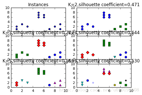
plt.subplot(3,2,1)

#初始化原始点
x1 = np.array([1,2,3,1,5,6,5,5,6,7,8,9,7,9])
x2 = np.array([1,3,2,2,8,6,7,6,7,1,2,1,1,3])
X = np.array(list(zip(x1,x2))).reshape(len(x1), 2)

#便于理解zip函数
print(list(x1))
print(list(x2))
print(list(zip(x1,x2)))
print(np.array(list(zip(x1,x2))).reshape(len(x1),2))

##在一号子图做出原始数据点阵分布
plt.xlim([0,10])
plt.ylim([0,10])
plt.title('Instances')
plt.scatter(x1,x2)

colors = ['b','g','r','c','m','y','k','b']
markets = ['o','s','D','v','^','p','*','+']

clusters = [2,3,4,5,8]
subplot_counter = 1
sc_scores = []

for t in clusters:
   subplot_counter += 1
   plt.subplot(3,2,subplot_counter)
   kmeans_model = KMeans(n_clusters=t).fit(X)
   print(kmeans_model.labels_)
   for i,l in enumerate(kmeans_model.labels_):
        plt.plot(x1[i],x2[i],color=colors[l],marker=markets[l],ls='None')
   plt.xlim([0,10])
   plt.ylim([0,10])
   sc_score=silhouette_score(X,kmeans_model.labels_,metric='euclidean')
   sc_scores.append(sc_score)
   plt.title('K=%s,silhouette coefficient=%0.03f'%(t,sc_score))

#绘制轮廓系数与不同类簇数量的关系曲线
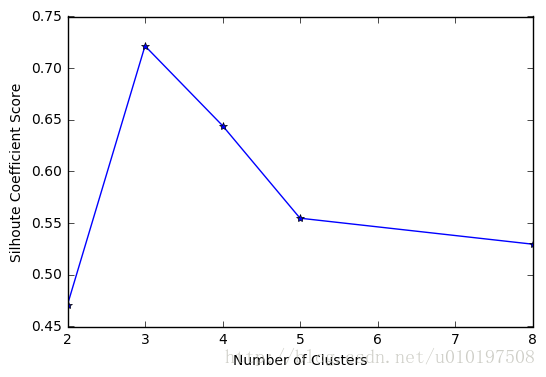
plt.figure()
print(clusters)
print(sc_scores)
plt.plot(clusters,sc_scores,'*-')
plt.xlabel('Number of Clusters')
plt.ylabel('Silhoute Coefficient Score')
plt.show()

0.6673881543921809
[1, 2, 3, 1, 5, 6, 5, 5, 6, 7, 8, 9, 7, 9]
[1, 3, 2, 2, 8, 6, 7, 6, 7, 1, 2, 1, 1, 3]
[(1, 1), (2, 3), (3, 2), (1, 2), (5, 8), (6, 6), (5, 7), (5, 6), (6, 7), (7, 1), (8, 2), (9, 1), (7, 1), (9, 3)]
[[1 1]
 [2 3]
 [3 2]
 [1 2]
 [5 8]
 [6 6]
 [5 7]
 [5 6]
 [6 7]
 [7 1]
 [8 2]
 [9 1]
 [7 1]
 [9 3]]
[0 0 0 0 0 0 0 0 0 1 1 1 1 1]
[1 1 1 1 2 2 2 2 2 0 0 0 0 0]
[2 2 2 2 1 1 1 1 1 3 0 0 3 0]
[2 3 3 2 1 1 1 1 1 0 4 4 0 4]
[3 0 7 3 4 2 4 2 4 5 1 1 5 6]
[2, 3, 4, 5, 8]
[0.47114752373147084, 0.72152991499839714, 0.64442490492524895, 0.5548170502705031, 0.52967730106134192]

import numpy as np
from sklearn.cluster import KMeans
from scipy.spatial.distance import cdist
import matplotlib.pyplot as plt

'''
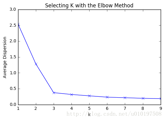
肘部观察法用于粗略预估相对合理的类簇个数
'''

#使用均匀分布函数随机三个簇，每个簇周围10个数据样本
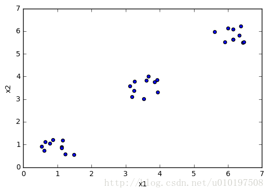
cluster1 = np.random.uniform(0.5,1.5,(2,10))
cluster2 = np.random.uniform(5.5,6.5,(2,10))
cluster3 = np.random.uniform(3.0,4.0,(2,10))

#绘制30个样本数据的分布图像
X = np.hstack((cluster1,cluster2,cluster3)).T
# print(cluster1)
# print(cluster2)
# print(cluster3)
# #print(np.hstack((cluster1,cluster2,cluster3)))
# print(np.hstack((cluster1,cluster2,cluster3)).T)
print(X[:,0])
plt.scatter(X[:,0],X[:,1])
plt.xlabel('x1')
plt.ylabel('x2')
plt.show()

#测试9种不同聚类中心数量下，每种情况下聚类的质量，并作图
K = range(1,10)
meandistortions = []

for k in K:
    kmeans = KMeans(n_clusters=k)
    kmeans.fit(X)
    meandistortions.append(sum(np.min(cdist(X,kmeans.cluster_centers_,'euclidean'),axis=1))/X.shape[0])

plt.plot(K,meandistortions,'bx-')
plt.xlabel('k')
plt.ylabel('Average Dispersion')
plt.title('Selecting K with the Elbow Method')
plt.show()

[ 0.52947724  1.12378755  1.48903264  0.63811499  1.15518886  0.87269295
  1.12656317  0.77838813  1.2324915   0.61778078  6.43504759  6.14920887
  6.46473326  6.33166436  6.14423172  5.91243809  5.9970971   6.38277121
  5.61600533  6.15116053  3.60959472  3.92813639  3.8515976   3.25619766
  3.18153509  3.12808213  3.93685184  3.24918762  3.66471859  3.53481055]