


- The cross-entropy cost function
- Introducing the cross-entropy cost function
- Using the cross-entropy to classify MNIST digits
- What does the cross-entropy mean Where does it come from
- Softmax
- Overfitting and regularization
- Regularization
- Why does regularization help reduce overfitting
- Other techniques for regularization
- Weight initialization
- Handwriting recognition revisited the code
- How to choose a neural networks hyper-parameters
- Other techniques
Backpropagation算法是神经网络训练的基础,本章介绍了一些技术来改进初始的backpropagation,内容包括:更好的cost function(the cross-entropy),四种regularization方法(L1 and L2 regularization, dropout, and artificial expansion of the training data),更好的权重初始化方法,选择hyper-parameters的启发式方法。
本章内容繁杂,但最终目的都是更好更快地训练一个神经网络。
The cross-entropy cost function
本节由练钢琴的例子引出通常在指出错误的情况下人类学习地更快。因此我们希望神经网络在出错的情况下学习地更快。
但实际中并非如此,由以下”玩具“例子说明:

用梯度下降法来训练这个神经元,实现输入1,输出为0。学习率为0.15。
假设初始权重为0.6,初始偏差为0.9。可知神经元初始的输出为0.82。
训练过程:

这个训练过程很合理,结果也算接近0。
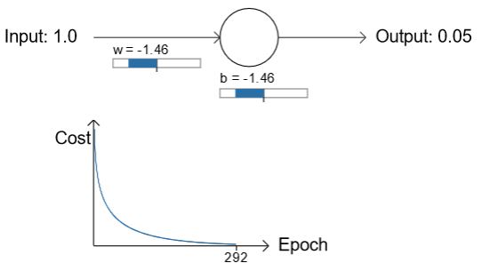
但是如果初始的权重和偏差都为2.0,初始的输出为0.98,训练曲线将如下:
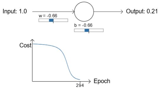
图中可见,虽然学习率不变,但是在开始的时候,也就是神经网络错的非常厉害的时候,cost function下降地非常慢,网络学习地非常慢。这与刚开始提出的学钢琴常识是相矛盾的。
为了解决这个矛盾,考虑我们的神经元学习是通过改变weight和bias实现的,而改变的rate是cost function的偏导
∂C/∂w
和
∂C/∂b
。所以网络学得非常慢意味着偏导的值非常小。我们使用的是quadratic cost function:
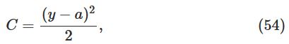
其中
a
是神经元的输出,为了写出偏导,由
因此考虑
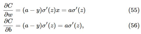
σ′(z)
,其为sigmoid function的斜率:

图中可以知道,当神经元输出接近1时,其斜率非常小,因此由如上推导出来的偏导
∂C/∂w
和
∂C/∂b
也非常小。这在初始的时候,输出接近1,直接导致了训练非常慢。
推广到一般情况,普遍的神经网络都是由此原因导致训练变慢的。
Introducing the cross-entropy cost function
将quadratic cost function替换成the cross-entropy可以解决上述的训练速度慢的问题。
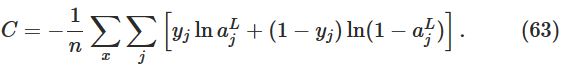
The cross-entropy cost function定义如下:
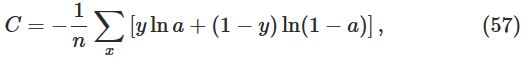
其中
n
是训练数据的个数,
有两个性质使得cross-entropy作为cost function是合理的:
首先,非负性,
C>0
。注意到所有
yln(a)+(1−y)ln(1−a)
都为负,加一个符号就为正了。
第二,如果神经元对所有输入样例
x
,输出都很接近desired output,此时cross-entropy将会接近0。
这两个性质是我们期望cost function的性质。quadratic cost function也有这两个性质,但cross-entropy避免了学习过慢的问题。
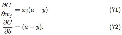
计算cross-entropy的偏导,并使用chainr rule,可以得到:
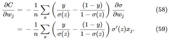
整理可得:
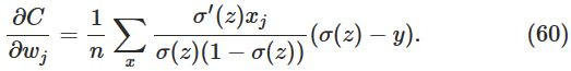
已知,
带入上式,可消项得:
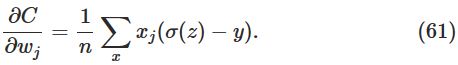
这个式子告诉我们,weight改变的rate由
σ(z)−y
来控制,也就是说由输出的误差来控制。误差越大,学得越快,这恰好就是在开头所述的学钢琴常识。而完成这些的原因在于cross-entropy使得
σ′
在化简中消项了。正是由于消去了激活函数的偏导项,才达到了优化初始学习速度慢的目的。
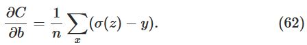
同样的,bias为:
用cross-entropy替代quadratic之后,初始化weight和bias都为2.0的例子,在初始时学习地不再那么慢了,并且输出也更接近0了:
多层输出的cross-entropy:
通常情况下,cross-entropy优于quadratic。
Using the cross-entropy to classify MNIST digits
What does the cross-entropy mean? Where does it come from?
这节解释了一下cross-entropy的意义,并讲解了cross-entropy是如何被想到的。
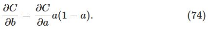
假设我们刚发现初始学习速度慢的问题,并发现了原因在于weight和bias偏导中的
σ′(z)
项。于是便有了消去这一项的想法。即有没有可能使得偏导转换为如下形式:
如果能够选择合适的cost function使得上式成立,那么就有可能解决问题。
为了求得满足上式的cost function,由chain rule,我们有:
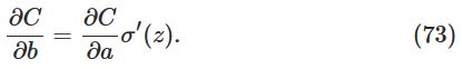
由于
σ′(z)=σ(z)(1−σ(z))=a(1−a)
,上式可以写为:
将(72)式带入上式,可得:

对其积分,得到:

即可得到cross-entropy的函数:
这节最后提了一下这种cross-entropy的表达式,是来自于信息论的,就是当结果和期望偏差很大时,我们会感到surprise;当结果和期望相近时,我们不会感到surprise。信息论中对surprise有明确的定义。
扩展阅读:(https://en.wikipedia.org/wiki/Cross_entropy#Motivation)
Softmax
这节简要介绍了另一种可以解决learning slowdown的方法-神经元的softmax层。
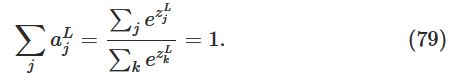
softmax的想法是为我们的神经网络定义一个新类型的输出层。在输出层,我们将不使用sigmoid函数,而是:
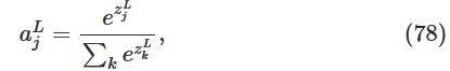
其中分母是所有输出元的和。
经过softmax的输出,首先其不会改变输入
z
的大小,
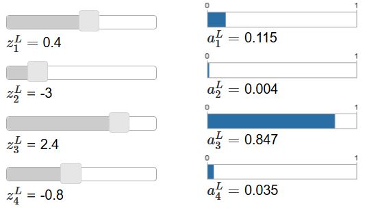
其次是经过输出后,其和为1,且输出全为正,如下:
也就是说,softmax层的输出可以认为是一个概率分布。因此在许多问题中,可以很方便的使用
aLj
来表示输出为
j
的概率。
Overfitting and regularization
这节介绍了过拟合问题。减小过拟合的方法之一是增加数据量。
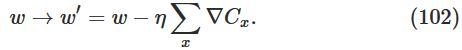
Regularization
Weight decay(L2 regularization)
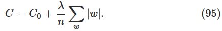
L2 regularization的思想是在cost function中多增加一项来限制weight的大小,比如cross-entropy:
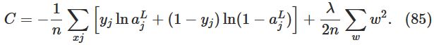
其中第二项是网络中所有weight的平方和,
一般的,可以将regularized cost function写成如下形式:
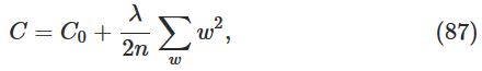
当
λ
较小的时候,我们希望original cost function比较小;当其比较大的时候,我们希望weight比较小。
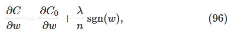
现在考虑如何将regularization用在SGD中,求其偏导,可得:
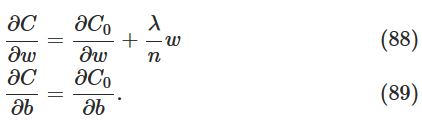
式中
∂C0/∂w
和
∂C0/∂b
项能使用backpropagation计算。
因此weight和bias的更新法则变为:
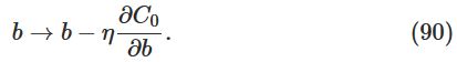
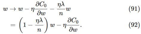
上式与原来的cost function不同点在于weight乘上了一个系数 1−ηλ/n ,这也正式其称为weight decay的原因,因为这个系数使得weight变小了。
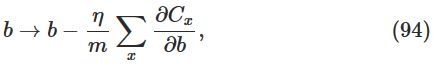
size为m的mini-batch更新法则:

regularization不仅可以减小过拟合和提升分类正确度,还可以避免训练时陷入local minima。
Why does regularization help reduce overfitting?
这节用一个拟合一次函数的例子说明了为什么regularization对过拟合有作用。
因为权重可以控制阶次,加入权重的限制,当权重接近0时,相当于当前高次项不存在了。
Other techniques for regularization
本节介绍了另外三种减小过拟合的方法。
L1 regularization
其形式如下:
原理和L2 regularization相同,可以减小权重。但其也有不同之处。
如果用上式训练神经网络,可得偏导:
Dropout
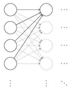
Dropout并不改变cost function,而是修改网络自身。比如如下网络:
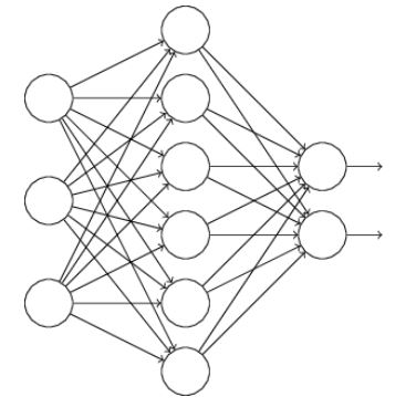
在dropout中,我们随机隐藏一半的神经元进行训练,比如下图就是一种:

我们对其训练之后得到了适合的weights和biases。然后对原来完整的神经网络再随机隐藏一半的神经元,再训练。在进行多次上述过程之后,我们的神经网络将会学习出很多组的weights和biases。最终将这些组的weights和biases集成起来(取均值)就是最终的神经网络。
对于dropout能解决过拟合,我的理解是,随机去除一些神经元,能减小神经网络所代表的“函数”的复杂程度。在NTU的DL课程中,老师用了人类神经网络成长的过程来说明这种方法是很有客观规律启发性的:
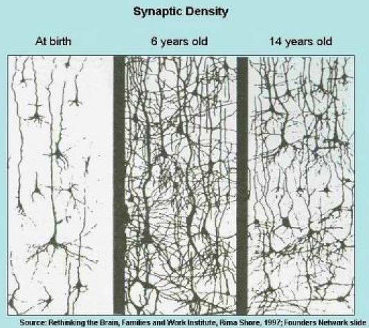
并且,从最终结果上来看,dropout与L1和L2 regularization很相似。
Artificially expanding the training data
实验表明,拥有更多的training data,将会得到better performance。
这节介绍了如何获得更多的数据,在实际中想要获得更多的数据往往花费很大,因此可以以人为的扩大数据集。
比如一张如下的数字5:

将其旋转一个小角度,比如15度:

这样就能获得一个新的label也为5的数据了。
我们可以用这种方法来扩大数据集,这种方法是很灵活的。比如在speech recognization中,可以通过加背景噪音等增加数据集。
An aside on big data and what it means to compare classification accuracies
这节比较了neural networks和SVM,并阐述了不要囿于在更佳的数据集上表现地更优越的算法,要大局比较。
Summing up
过拟合是训练中出现的主要要问题,由于计算机的性能提高,使得巨大的神经网络训练成为可能,大数据计算成为可能。因此,regularization十分重要。
Weight initialization
在建立神经网络的时候,我们需要初始化weights和biases。
在第一章时,我们初始化的方式是使用独立高斯随机变量初始化,高斯分布的均值为0,方差为1。虽然这种方法还不错,但是我们尝试着寻找一种更好的方法初始化,来使得我们的神经网络训练更快。
事实证明,我们可以比normalized Gaussians初始化做的更好。假设我们训练一个非常大的神经网络,有1000个输入神经元。假设我们用normalized Gaussian来初始化链接到第一个隐藏层的weights。现在注意力集中到第一个隐藏层的第一个元素:
为了简便,设输入的数据有一半为1,一半为0。因此
z=∑jwjxj+b
只有501项,因此
z
也为一个均值为0,标准差为
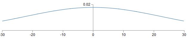
从图中可以看到
在早先时候,我们用改变cost function的方式解决了学习过慢的问题,但是改变cost function只会帮助saturated output neurons,并不会对saturated hidden neurons有任何帮助。
因此,提出了更好的初始化方法:
假设我们有
nin
个输入weights的神经元,我们将weights初始化为均值为0,标准差为
1/nin−−−√
的随机高斯分布变量。
继续使用上述例子,我们将会得到一个均值为0,标准差为
3/2−−−√=1.22
的高斯分布:
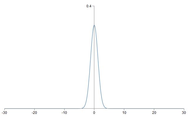
这样输出的
z
就不容易使得
对于bias,原先的初始化方案影响不大,因此依旧使用原先的初始化方案。
Handwriting recognition revisited: the code
这节将这一章所讨论过的方法修改第一章的代码。
首先回顾几个点:
np.random.randn(y, x),表示的是生成一个y行x列的服从均值 μ 为0,方差 σ2 为1的高斯分布。
zip(x,y),可以将x与y的元素一一对应成为一个tuple。
np.nan_to_num,保证了在处理非常接近0时的log函数是正确的。
完整代码如下:
"""network2.py
~~~~~~~~~~~~~~

An improved version of network.py, implementing the stochastic
gradient descent learning algorithm for a feedforward neural network.
Improvements include the addition of the cross-entropy cost function,
regularization, and better initialization of network weights.  Note
that I have focused on making the code simple, easily readable, and
easily modifiable.  It is not optimized, and omits many desirable
features.

"""

#### Libraries
# Standard library
import json
import random
import sys

# Third-party libraries
import numpy as np


#### Define the quadratic and cross-entropy cost functions

class QuadraticCost(object):

    @staticmethod
    def fn(a, y):
        """Return the cost associated with an output ``a`` and desired output
        ``y``.

        """
        return 0.5*np.linalg.norm(a-y)**2

    @staticmethod
    def delta(z, a, y):
        """Return the error delta from the output layer."""
        return (a-y) * sigmoid_prime(z)


class CrossEntropyCost(object):

    @staticmethod
    def fn(a, y):
        """Return the cost associated with an output ``a`` and desired output
        ``y``.  Note that np.nan_to_num is used to ensure numerical
        stability.  In particular, if both ``a`` and ``y`` have a 1.0
        in the same slot, then the expression (1-y)*np.log(1-a)
        returns nan.  The np.nan_to_num ensures that that is converted
        to the correct value (0.0).

        """
        return np.sum(np.nan_to_num(-y*np.log(a)-(1-y)*np.log(1-a)))

    @staticmethod
    def delta(z, a, y):
        """Return the error delta from the output layer.  Note that the
        parameter ``z`` is not used by the method.  It is included in
        the method's parameters in order to make the interface
        consistent with the delta method for other cost classes.

        """
        return (a-y)


#### Main Network class
class Network(object):

    def __init__(self, sizes, cost=CrossEntropyCost):
        """The list ``sizes`` contains the number of neurons in the respective
        layers of the network.  For example, if the list was [2, 3, 1]
        then it would be a three-layer network, with the first layer
        containing 2 neurons, the second layer 3 neurons, and the
        third layer 1 neuron.  The biases and weights for the network
        are initialized randomly, using
        ``self.default_weight_initializer`` (see docstring for that
        method).

        """
        self.num_layers = len(sizes)
        self.sizes = sizes
        self.default_weight_initializer()
        self.cost=cost

    def default_weight_initializer(self):
        """Initialize each weight using a Gaussian distribution with mean 0
        and standard deviation 1 over the square root of the number of
        weights connecting to the same neuron.  Initialize the biases
        using a Gaussian distribution with mean 0 and standard
        deviation 1.

        Note that the first layer is assumed to be an input layer, and
        by convention we won't set any biases for those neurons, since
        biases are only ever used in computing the outputs from later
        layers.

        """
        self.biases = [np.random.randn(y, 1) for y in self.sizes[1:]]
        self.weights = [np.random.randn(y, x)/np.sqrt(x)
                        for x, y in zip(self.sizes[:-1], self.sizes[1:])]

    def large_weight_initializer(self):
        """Initialize the weights using a Gaussian distribution with mean 0
        and standard deviation 1.  Initialize the biases using a
        Gaussian distribution with mean 0 and standard deviation 1.

        Note that the first layer is assumed to be an input layer, and
        by convention we won't set any biases for those neurons, since
        biases are only ever used in computing the outputs from later
        layers.

        This weight and bias initializer uses the same approach as in
        Chapter 1, and is included for purposes of comparison.  It
        will usually be better to use the default weight initializer
        instead.

        """
        self.biases = [np.random.randn(y, 1) for y in self.sizes[1:]]
        self.weights = [np.random.randn(y, x)
                        for x, y in zip(self.sizes[:-1], self.sizes[1:])]

    def feedforward(self, a):
        """Return the output of the network if ``a`` is input."""
        for b, w in zip(self.biases, self.weights):
            a = sigmoid(np.dot(w, a)+b)
        return a

    def SGD(self, training_data, epochs, mini_batch_size, eta,
            lmbda = 0.0,
            evaluation_data=None,
            monitor_evaluation_cost=False,
            monitor_evaluation_accuracy=False,
            monitor_training_cost=False,
            monitor_training_accuracy=False):
        """Train the neural network using mini-batch stochastic gradient
        descent.  The ``training_data`` is a list of tuples ``(x, y)``
        representing the training inputs and the desired outputs.  The
        other non-optional parameters are self-explanatory, as is the
        regularization parameter ``lmbda``.  The method also accepts
        ``evaluation_data``, usually either the validation or test
        data.  We can monitor the cost and accuracy on either the
        evaluation data or the training data, by setting the
        appropriate flags.  The method returns a tuple containing four
        lists: the (per-epoch) costs on the evaluation data, the
        accuracies on the evaluation data, the costs on the training
        data, and the accuracies on the training data.  All values are
        evaluated at the end of each training epoch.  So, for example,
        if we train for 30 epochs, then the first element of the tuple
        will be a 30-element list containing the cost on the
        evaluation data at the end of each epoch. Note that the lists
        are empty if the corresponding flag is not set.

        """
        if evaluation_data: n_data = len(evaluation_data)
        n = len(training_data)
        evaluation_cost, evaluation_accuracy = [], []
        training_cost, training_accuracy = [], []
        for j in xrange(epochs):
            random.shuffle(training_data)
            mini_batches = [
                training_data[k:k+mini_batch_size]
                for k in xrange(0, n, mini_batch_size)]
            for mini_batch in mini_batches:
                self.update_mini_batch(
                    mini_batch, eta, lmbda, len(training_data))
            print "Epoch %s training complete" % j
            if monitor_training_cost:
                cost = self.total_cost(training_data, lmbda)
                training_cost.append(cost)
                print "Cost on training data: {}".format(cost)
            if monitor_training_accuracy:
                accuracy = self.accuracy(training_data, convert=True)
                training_accuracy.append(accuracy)
                print "Accuracy on training data: {} / {}".format(
                    accuracy, n)
            if monitor_evaluation_cost:
                cost = self.total_cost(evaluation_data, lmbda, convert=True)
                evaluation_cost.append(cost)
                print "Cost on evaluation data: {}".format(cost)
            if monitor_evaluation_accuracy:
                accuracy = self.accuracy(evaluation_data)
                evaluation_accuracy.append(accuracy)
                print "Accuracy on evaluation data: {} / {}".format(
                    self.accuracy(evaluation_data), n_data)
            print
        return evaluation_cost, evaluation_accuracy, \
            training_cost, training_accuracy

    def update_mini_batch(self, mini_batch, eta, lmbda, n):
        """Update the network's weights and biases by applying gradient
        descent using backpropagation to a single mini batch.  The
        ``mini_batch`` is a list of tuples ``(x, y)``, ``eta`` is the
        learning rate, ``lmbda`` is the regularization parameter, and
        ``n`` is the total size of the training data set.

        """
        nabla_b = [np.zeros(b.shape) for b in self.biases]
        nabla_w = [np.zeros(w.shape) for w in self.weights]
        for x, y in mini_batch:
            delta_nabla_b, delta_nabla_w = self.backprop(x, y)
            nabla_b = [nb+dnb for nb, dnb in zip(nabla_b, delta_nabla_b)]
            nabla_w = [nw+dnw for nw, dnw in zip(nabla_w, delta_nabla_w)]
        self.weights = [(1-eta*(lmbda/n))*w-(eta/len(mini_batch))*nw
                        for w, nw in zip(self.weights, nabla_w)]
        self.biases = [b-(eta/len(mini_batch))*nb
                       for b, nb in zip(self.biases, nabla_b)]

    def backprop(self, x, y):
        """Return a tuple ``(nabla_b, nabla_w)`` representing the
        gradient for the cost function C_x.  ``nabla_b`` and
        ``nabla_w`` are layer-by-layer lists of numpy arrays, similar
        to ``self.biases`` and ``self.weights``."""
        nabla_b = [np.zeros(b.shape) for b in self.biases]
        nabla_w = [np.zeros(w.shape) for w in self.weights]
        # feedforward
        activation = x
        activations = [x] # list to store all the activations, layer by layer
        zs = [] # list to store all the z vectors, layer by layer
        for b, w in zip(self.biases, self.weights):
            z = np.dot(w, activation)+b
            zs.append(z)
            activation = sigmoid(z)
            activations.append(activation)
        # backward pass
        delta = (self.cost).delta(zs[-1], activations[-1], y)
        nabla_b[-1] = delta
        nabla_w[-1] = np.dot(delta, activations[-2].transpose())
        # Note that the variable l in the loop below is used a little
        # differently to the notation in Chapter 2 of the book.  Here,
        # l = 1 means the last layer of neurons, l = 2 is the
        # second-last layer, and so on.  It's a renumbering of the
        # scheme in the book, used here to take advantage of the fact
        # that Python can use negative indices in lists.
        for l in xrange(2, self.num_layers):
            z = zs[-l]
            sp = sigmoid_prime(z)
            delta = np.dot(self.weights[-l+1].transpose(), delta) * sp
            nabla_b[-l] = delta
            nabla_w[-l] = np.dot(delta, activations[-l-1].transpose())
        return (nabla_b, nabla_w)

    def accuracy(self, data, convert=False):
        """Return the number of inputs in ``data`` for which the neural
        network outputs the correct result. The neural network's
        output is assumed to be the index of whichever neuron in the
        final layer has the highest activation.

        The flag ``convert`` should be set to False if the data set is
        validation or test data (the usual case), and to True if the
        data set is the training data. The need for this flag arises
        due to differences in the way the results ``y`` are
        represented in the different data sets.  In particular, it
        flags whether we need to convert between the different
        representations.  It may seem strange to use different
        representations for the different data sets.  Why not use the
        same representation for all three data sets?  It's done for
        efficiency reasons -- the program usually evaluates the cost
        on the training data and the accuracy on other data sets.
        These are different types of computations, and using different
        representations speeds things up.  More details on the
        representations can be found in
        mnist_loader.load_data_wrapper.

        """
        if convert:
            results = [(np.argmax(self.feedforward(x)), np.argmax(y))
                       for (x, y) in data]
        else:
            results = [(np.argmax(self.feedforward(x)), y)
                        for (x, y) in data]
        return sum(int(x == y) for (x, y) in results)

    def total_cost(self, data, lmbda, convert=False):
        """Return the total cost for the data set ``data``.  The flag
        ``convert`` should be set to False if the data set is the
        training data (the usual case), and to True if the data set is
        the validation or test data.  See comments on the similar (but
        reversed) convention for the ``accuracy`` method, above.
        """
        cost = 0.0
        for x, y in data:
            a = self.feedforward(x)
            if convert: y = vectorized_result(y)
            cost += self.cost.fn(a, y)/len(data)
        cost += 0.5*(lmbda/len(data))*sum(
            np.linalg.norm(w)**2 for w in self.weights)
        return cost

    def save(self, filename):
        """Save the neural network to the file ``filename``."""
        data = {"sizes": self.sizes,
                "weights": [w.tolist() for w in self.weights],
                "biases": [b.tolist() for b in self.biases],
                "cost": str(self.cost.__name__)}
        f = open(filename, "w")
        json.dump(data, f)
        f.close()

#### Loading a Network
def load(filename):
    """Load a neural network from the file ``filename``.  Returns an
    instance of Network.

    """
    f = open(filename, "r")
    data = json.load(f)
    f.close()
    cost = getattr(sys.modules[__name__], data["cost"])
    net = Network(data["sizes"], cost=cost)
    net.weights = [np.array(w) for w in data["weights"]]
    net.biases = [np.array(b) for b in data["biases"]]
    return net

#### Miscellaneous functions
def vectorized_result(j):
    """Return a 10-dimensional unit vector with a 1.0 in the j'th position
    and zeroes elsewhere.  This is used to convert a digit (0...9)
    into a corresponding desired output from the neural network.

    """
    e = np.zeros((10, 1))
    e[j] = 1.0
    return e

def sigmoid(z):
    """The sigmoid function."""
    return 1.0/(1.0+np.exp(-z))

def sigmoid_prime(z):
    """Derivative of the sigmoid function."""
return sigmoid(z)*(1-sigmoid(z))注意到以上代码用JSON而不是python的pickle和cPickle来保存和读取。因为如果未来我们要改动一个神经元,我们改动的是代码Network._init_的方法。如果我们用pickle来读取,我们可能会失败。用JSON来保存使得旧的Networks仍旧可以load。
How to choose a neural network’s hyper-parameters?
本节主要介绍了如何选择参数,比如learning rate η ,regularization parameter λ 等等。
Broad strategy
刚开始建立一个神经网络的时候,可以先缩小问题的范围,达到快速训练的目的。也可以在开始的时候选择一个小一点的神经网络来训练。还可以增加frequency of monitoring。
Learning rate
如下图:
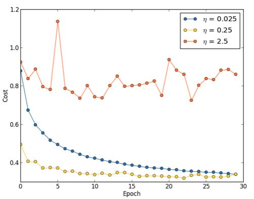
如果
η
过大会步伐太大,以至于波动,而如果过小,则会造成训练缓慢。记得在斯坦福Ng的课程里面,他是用一个二次函数来演示如何选择learning rate的。还记得当时选用的步长是0.3。
而这里的建议是,首先估计一个
η
的threshold value,就是当cost开始下降,而不是振荡或者上升的那个值,这个估计不需要太精确;我个人觉得招到这个值之后可以使用二分来调参,因为这个参数是有指向性的,而本节则是用缩小十倍十倍的方法。
Use early stopping to determine the number of training epochs
提早停止要求每个循环都计算validation data的准确度,提早停止也能防止过拟合。
准确的说,提早停止是指,当准确度已经不再上升了就可以停止了。
Learning rate schedule
之前我们都使得learning rate为constant,但是我们可以让learning rate随着训练的加深而变化。即在训练开始时,可以使用较大的学习率,之后慢慢减小。
The regularization parameter
这里的建议是,先将 λ 设为0,然后确定学习率 η 的值,然后用validation data来设定 λ ,
Mini-batch size
本节说明了如何设置mini-batch的大小,首先假设我们在做online learning,也就是说,把mini-batch size设为1。
很明显的将会出错的地方在于每次只用一个训练样例,会导致错误的gradient估计。但事实上单个gradient的估计不需要非常准确,只要每次使得cost function值下降就行了。
基于这个说法,好像我们使用的是online learning,但实际上更复杂。上一章指出,可以用矩阵的技术来计算所有在mini-batch中的样例gradient的更新,而不是跑循环。依赖硬件和线性代数函数库,这样做可以使得计算gradient更加快速。这个说法已经在之前的vectorization中提到过了。
现在,假设mini-batch为100,其更新规则为:
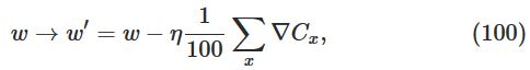
其中的和为所有在mini-batch中训练样例的和。
这与online learning不同,online learning的更新规则:

但如果我们将mini-batch中的learning rate提高一百倍,可以得到:
这看起来和online learning很像,但是时间花费是远远高于online learning的。
讲道理,这几段我没读懂用意是什么。记一下结论吧:
如果mini-batch的size太小,那么硬件优势和好的线性代数库函数的加速将不会太多;如果太大了,更新weights的频率将会很低。最优的值将会使得神经网络有最大的学习速度。幸运的是使得训练速度最快的mini-batch的size和其他的hyper-parameters无关,因此并不需要优化这些参数来寻找一个好的mini-batch的size。
选择mini-batch的方法:
为其他的hyper-parameters选择一些可接受的数值,然后尝试一系列不同的mini-batch size,同时像之前那样scaling
η
;然后比较validation accuracy的time(真实的时间,而不是epoch),选择最快的那个。用这个mini-batch size来选择其他的hyper-parameters。
Automated techniques
以上的技巧全是手动设置参数,手动设置参数可以让我们学习到一个神经网络是如何工作的。但让这些过程自动工作的方法也是存在的,比如grid search,还有其他很多的方法。
Summing up
以上的方法都是rules of thumb(经验法则),而不是rules cast in stone。实际中常常调参数是反反复复的工作,每个参数都要前后调整。我们需要的是小心地对待网络不能很好工作的迹象,并且愿意实验。要注意网络的behaviour,特别是validation accuracy。
Other techniques
这一节介绍的技术不仅仅是为了了解,而是为了熟悉一些常常会出现在神经网络中的问题和如何解决他们。
Variations on stochastic gradient descent
虽然SGD在我们的手写识别例子中已经很好了。但还有很多不同的方法来optimizing the cost function。有时他们的表现更好。
Hessian technique
这里我们讨论一个抽象的问题:
最小化一个变量为
w=w1,w2,...
的代价函数
C
,使得
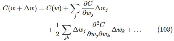
可以将上式写为:

上式
∇
是gradient vector;H是Hessian matrix,其第
jk
个元素为
∂2C/∂wj∂wk
。
省略上式的高次项,上式可以写为:

计算后,我们发现上式右边可以由下式的选择最小化:
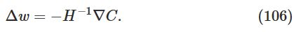
因此(105)式可以作为一个好的cost function。我们可以有以下更新方法:
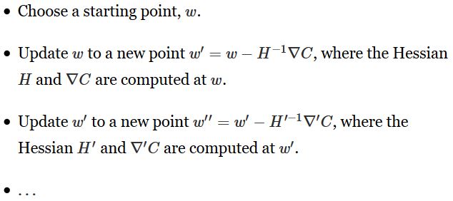
实际中,用的是一下形式,加上了learning rate:
这种方法叫Hessian technique 或 Hessian optimization。实验表明,这种方法比标准的gradient descent收敛时间更短。并且计算Hessian矩阵有很多方法。
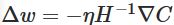
虽然理论上Hessian optimization很好,但它却很难用在实际中。因为Hessian矩阵实在是太大了,比如一个神经网络有 107 个weights和biases,则Hessian矩阵将会有 1014 个元素。计算 H−1∇C 太难了。
Momentum-based gradient descent
这种方法和上述方法差不多,但是它避免了大量的矩阵二次求导的计算。
为了理解这种方法,我们回到本章开始的小球图:
在NTU课程里面已经见识过这种方法了,就是给小球加上惯性,使其表现地更像物理场景,当时给的优点是可以避免陷入local minima。
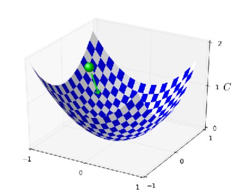
而这里则是给系统加上了摩擦力。假设速度变量
v=v1,v2,...
对应
wj
。替换原先的:

为:
其中,
μ
是一个控制摩擦力的系数。为了理解上式,先考虑
μ=1
的情况,代表没有摩擦力。此时表示”力”
∇C
驱动速度
v
,速度控制
momentum技术普遍地用在学习的加速上。它的优势是即可以用backpropagation来计算gradients,还可以抽样随机选择mini-batches,从Hessian技术中取长,看出gradient怎么改变的。
Other approaches to minimizing the cost function
有许多其他的技术,要了解其优缺点。
Other models of artificial neuron
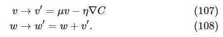
这节介绍了其他一些可能相比sigmoid更优秀的激活函数。
首先是tanh函数:
经过一些数学计算,可以得到:
可知tanh函数是一种rescaled版本的sigmoid函数。
其函数图像如下:
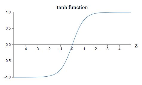
那么二者间谁好呢?有些研究表明tanh有时会表现地好一点。假设我们使用sigmoid,因此神经网络中所有的
a
都为正的。考虑
但在实际中,我们没有办法权衡哪个函数更加优秀一点。
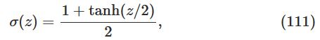
另一个是rectified linear neuron 或者 rectified linear unit函数,简称ReLU。
其形式为:

函数图像为:
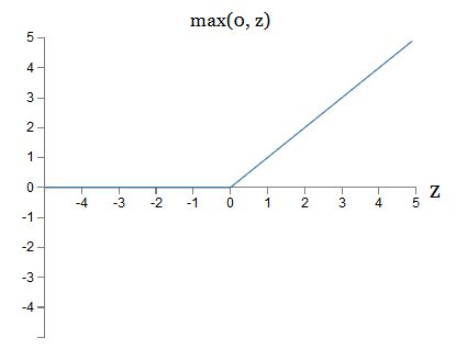
显然这种函数和tanh、sigmoid函数特别不一样。可是它也可以表示出任意函数,并且在backpropagation中也可以训练。
什么时候能用到ReLU?在最近的关于图像识别的研究中发现ReLU很有用。但与tanh不同,我们不能确切的知道它应该在什么时候使用。回想之前的sigmoid会在饱和的时候停止学习,也就是说在其输出值接近0或1的时候停止学习。在这章我们已经学到,这是因为
现在我们有很多强有力的工具在手中了。


 1634
1634

 被折叠的 条评论
为什么被折叠?
被折叠的 条评论
为什么被折叠?
 到【灌水乐园】发言


