CNN卷积神经网络

CNN是一种多层神经网络，基于人工神经网络，在人工神经网络前，用滤波器进行特征抽取，使用卷积核作为特征抽取器，自动训练特征抽取器，就是说卷积核以及阈值参数这些都需要由网络去学习。

图像可以直接作为网络的输入，避免了传统识别算法中复杂的特征提取和数据重建过程。

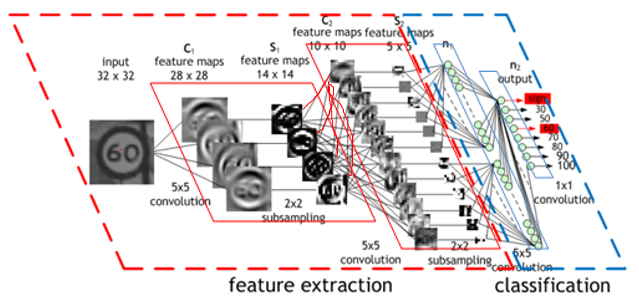
一般卷积神经网络的结构：

前面feature extraction部分体现了CNN的特点，feature extraction部分最后的输出可以作为分类器的输入。这个分类器你可以用softmax或RBF等等。

局部感受野与权值共享

局部感受野指卷基层的神经元只和上一层map的局部窗口相联系。

权值共享指每一个map都由一个卷积核去做卷积得到。

权值共享减少了权值数量，降低了网络复杂度。

Conv layer

卷积层中的每个神经元提取前一层若干特征图中相同位置的局部特征。设卷积层为第i层，该层的第j个特征图为Oij，则Oij的元素Oij(x,y)为：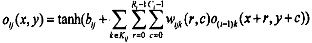

其中，tanh(·)是双曲正切函数，bij为属于特征图Oij的可训练偏置，Kij为与Oij相连的第i-1层中特征图标号的集合。Wijk是连接特征图Oij和特征图O(i-1)k的卷积核窗口，Ri和Ci分别为该层卷积核的行数和列数。若第i-l层特征图的大小为n1×n2，连接第i-1层特征图和第i层特征图的卷积核大小为I1×12，则第i层特征图的大小为(n1-l1+1)×(n2-l2+1)．

Subsampling  layer

子采样层中的每个特征图唯一对应前一层的一个特征图，各特征图组合前一层对应特征图巾大小相同但互不重叠的所有子区域，使得卷积神经网络具有一定的空间不变性，从而实现一定程度的shift 和 distortion invariance。利用图像局部相关性的原理，对图像进行子抽样，可以减少数据处理量同时保留有用信息。这个过程也被称为pooling，常用pooling 有两种：

mean-pooling、max-pooling。

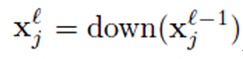
down(X_j^l-1)表示下采样操作，就是对一个小区域进行pooling操作，使数据降维。

有的算法还会对mean-pooling、max-pooling后的输出进行非线性映射

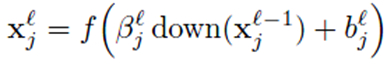
f是激活函数。

Evaluation of Pooling Operations in. Convolutional Architectures for Object Recognition这篇文献证明了最大池一般效果更好。

貌似现在已经有用histogram做pooling的了。

注意，卷积的计算窗口是有重叠的，而采用的计算窗口没有重叠。

关于激活函数的选择

一般来说深度神经网络中的激活函数选用RELU而不用sigmoid或tanh。

ReLU(x)=max(x,0)

原因如下：

链接：http://www.zhihu.com/question/29021768/answer/43488153
来源：知乎

第一，采用sigmoid等函数，反向传播求误差梯度时，求导计算量很大，而Relu求导非常容易。（这个不大认同，sigmoid求导可以直接给出公式：f'(x) = f(x)[1-f(x)]）

第二，对于深层网络，sigmoid函数反向传播时，很容易就会出现梯度消失的情况（在sigmoid接近饱和区时，变换太缓慢，导数趋于0），从而无法完成深层网络的训练。

第三，Relu会使一部分神经元的输出为0，这样就造成了网络的稀疏性，并且减少了参数的相互依存关系，缓解了过拟合问题的发生。

sigmoid和tanh函数的图像如下：

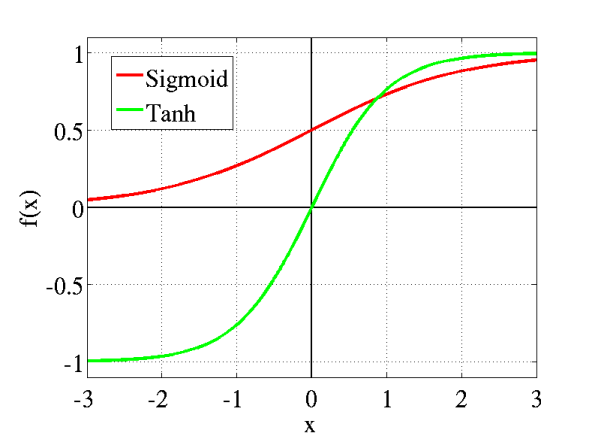
很自然的看到他们的导数两端接近0.

1. 传统的激励函数，计算时要用指数或者三角函数，计算量至少要比简单的 ReLU 高两个数量级；
2. ReLU 的导数是常数，非零即一，不存在传统激励函数在反向传播计算中的"梯度消失问题"；
3. 由于统计上，约一半的神经元在计算过程中输出为零，使用 ReLU 的模型计算效率更高，而且自然而然的形成了所谓 "稀疏表征" (sparse representation)，用少量的神经元可以高效，灵活，稳健地表达抽象复杂的概念。

ReLu的变体

noisy ReLUs

可将其包含Gaussian noise得到noisy ReLUs，f(x)=max(0,x+N(0,σ(x)))，常用来在机器视觉任务里的restricted Boltzmann machines中。

leaky ReLUs

允许小的非零的gradient 当unit没有被激活时。

f(x)={x0.01xif x>0otherwise

PRelu

[PRelu--Delving Deep into Rectifiers: Surpassing Human-Level Performance on ImageNet Classification.]

PRelu的表达式：

 

是Relu的增强版，PRelu使得模型在ImageNet2012上的结果提高到4.94%，超过普通人的正确率；PRelu需要像更新权重weights一样使用BP更新一个额外的参数，但是相较于weights的数量来说，PRelu需要更新的参数总数可以忽略不计，所以不会加重overfitting的影响。

如果PRelu的参数为0，那其实就是Relu；如果PRelu的参数为一个很小的常数constant，比如0.01,那其实就是Leaky Relu(LRelu)。

输出层

最后一个卷积-采样层的输出可作为输出层的输入，输出层是全连接层。输出层是一个权值可微的分类器，可以让整个网络使用基于梯度的学习方法来进行全局训练，比如softmax、RBF网络、 一层或两层的全连接神经网络等分类算法。但即使不可微的分类器（比如svm）其实也可以使用的，方法是先用可微的分类器调参数，参数调好后把分类器换掉就行了。

以LeNet5为例，其结构如下：

C1,C3,C5 : Convolutional layer. 
                 5 × 5 Convolution matrix.
S2 , S4 :    Subsampling layer.
                 Subsampling by factor 2.
F6 :           Fully connected layer

OUTPUT :  RBF

C层和S层成对出现，C承担特征抽取，S承担抗变形。C元中涉及两个重要参数，即感受野与阈值参数，前者确定输入连接的数目，后者则控制对特征子模式的反应程度。

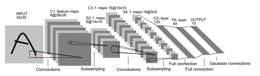
C1层是一个卷积层（通过卷积运算，可以增强图像的某种特征，并且降低噪音），由6个特征图Feature Map构成。Feature Map中每个神经元与输入中5*5的邻域相连。特征图的大小为28*28。C1有156个可训练参数（每个滤波器5*5=25个unit参数和一个bias参数，一共6个滤波器，共(5*5+1)*6=156个参数），共156*(28*28)=122,304个连接。

S2层是一个下采样层，有6个14*14的特征图。特征图中的每个单元与C1中相对应特征图的2*2邻域相连接。S2层每个单元的4个输入相加，乘以一个可训练参数，再加上一个可训练偏置。结果通过sigmoid函数计算。可训练系数和偏置控制着sigmoid函数的非线性程度。如果系数比较小，那么运算近似于线性运算，亚采样相当于模糊图像。如果系数比较大，根据偏置的大小亚采样可以被看成是有噪声的“或”运算或者有噪声的“与”运算。每个单元的2*2感受野并不重叠，因此S2中每个特征图的大小是C1中特征图大小的1/4（行和列各1/2）。S2层有12个可训练参数和5880个连接。

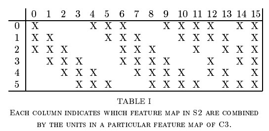
C3层也是一个卷积层，它同样通过5x5的卷积核去卷积层S2，然后得到的特征map就只有10x10个神经元，但是它有16种不同的卷积核，所以就存在16个特征map了。这里需要注意的一点是：C3中的每个特征map是连接到S2中的所有6个或者几个特征map的，表示本层的特征map是上一层提取到的特征map的不同组合。

S4层是一个下采样层，由16个5*5大小的特征图构成。特征图中的每个单元与C3中相应特征图的2*2邻域相连接，跟C1和S2之间的连接一样。S4层有32个可训练参数（每个特征图1个因子和一个偏置）和2000个连接。

C5层是一个卷积层，有120个特征图。每个单元与S4层的全部16个单元的5*5邻域相连。由于S4层特征图的大小也为5*5（同滤波器一样），故C5特征图的大小为1*1：这构成了S4和C5之间的全连接。之所以仍将C5标示为卷积层而非全相联层，是因为如果LeNet-5的输入变大，而其他的保持不变，那么此时特征图的维数就会比1*1大。C5层有48120个可训练连接。
F6层有84个单元（之所以选这个数字的原因来自于输出层的设计），与C5层全相连。有10164个可训练参数。如同经典神经网络，F6层计算输入向量和权重向量之间的点积，再加上一个偏置。然后将其传递给sigmoid函数产生单元i的一个状态。
最后，输出层由欧式径向基函数（Euclidean Radial Basis Function）单元组成，每类一个单元，每个有84个输入。换句话说，每个输出RBF单元计算输入向量和参数向量之间的欧式距离。输入离参数向量越远，RBF输出的越大。一个RBF输出可以被理解为衡量输入模式和与RBF相关联类的一个模型的匹配程度的惩罚项。用概率术语来说，RBF输出可以被理解为F6层配置空间的高斯分布的负log-likelihood。给定一个输入模式，损失函数应能使得F6的配置与RBF参数向量（即模式的期望分类）足够接近。这些单元的参数是人工选取并保持固定的（至少初始时候如此）。这些参数向量的成分被设为-1或1。虽然这些参数可以以-1和1等概率的方式任选，或者构成一个纠错码，但是被设计成一个相应字符类的7*12大小（即84）的格式化图片。

分类器中的全连接层需要以卷积的形式来实现，即以卷积核和输入大小一样的卷积操作来实现全连接。

卷积核和偏置的初始化

卷积核和偏置在开始时要随机初始化，这些参数是要在训练过程中学习的。卷积核[-sqrt(6 / (fan_in + fan_out)), sqrt(6 / (fan_in + fan_out))] 的取值范围选择来自于Bengio 的Understanding the difficulty of training deep feedforward neuralnetworks这篇文章。

卷积核的另一种初始化方法是用autoencoder去学习参数。

Caffe中用来初始化权值有如下表的类型：

类型	派生类	说明
constant	ConstantFiller	使用一个常数（默认为0）初始化权值
gaussian	GaussianFiller	使用高斯分布初始化权值
positive_unitball	PositiveUnitballFiller
uniform	UniformFiller	使用均为分布初始化权值
xavier	XavierFiller	使用xavier算法初始化权值
msra	MSRAFiller
bilinear	BilinearFiller

1 xavier

使用分布  x∼U(−3/n−−−√,+3/n−−−√)  初始化权值 w  为。总的来说 n 的值为输入输出规模相关，公式如下:

n=⎧⎩⎨⎪⎪⎪⎪⎪⎪fan_infan_in+fan_out2fan_outdefaultvariance_norm=AVERAGEvariance_norm=FAN_OUT

{fan_in=blob.count/blob.numfan_out=blob.count/blob.channels

前向传递

前向传递比较简单。

误差反向传导

卷积神经网络巾误差的反向传播分两步，一是输出层的误差反向传播，二是隐藏层的误差反向传播。

分割线间的内容来自：http://www.cnblogs.com/fengfenggirl/p/cnn_implement.html#refren1，解释得很好。

/******************************************************************************************************************************/

反向传输过程是CNN最复杂的地方，虽然从宏观上来看基本思想跟BP一样，都是通过最小化残差来调整权重和偏置，但CNN的网络结构并不像BP那样单一，对不同的结构处理方式不一样，而且因为权重共享，使得计算残差变得很困难，很多论文[1][5]和文章[4]都进行了详细的讲述，但我发现还是有一些细节没有讲明白，特别是采样层的残差计算，我会在这里详细讲述。

　　4.1输出层的残差

　　和BP一样，CNN的输出层的残差与中间层的残差计算方式不同，输出层的残差是输出值与类标值得误差值，而中间各层的残差来源于下一层的残差的加权和。输出层的残差计算如下：

公式来源

　　这个公式不做解释，可以查看公式来源，看斯坦福的深度学习教程的解释。

　　4.2 下一层为采样层（subsampling）的卷积层的残差

　　当一个卷积层L的下一层(L+1)为采样层，并假设我们已经计算得到了采样层的残差，现在计算该卷积层的残差。从最上面的网络结构图我们知道，采样层（L+1）的map大小是卷积层L的1/（scale*scale），ToolBox里面，scale取2，但这两层的map个数是一样的，卷积层L的某个map中的4个单元与L+1层对应map的一个单元关联，可以对采样层的残差与一个scale*scale的全1矩阵进行克罗内克积进行扩充，使得采样层的残差的维度与上一层的输出map的维度一致，Toolbox的代码如下，其中d表示残差，a表示输出值：

net.layers{l}.d{j} = net.layers{l}.a{j} .* (1 - net.layers{l}.a{j}) .* expand(net.layers{l + 1}.d{j}, [net.layers{l + 1}.scale net.layers{l + 1}.scale 1])

　　扩展过程：

图5

　　利用卷积计算卷积层的残差：

图6

　　4.3 下一层为卷积层（subsampling）的采样层的残差

　　当某个采样层L的下一层是卷积层(L+1)，并假设我们已经计算出L+1层的残差，现在计算L层的残差。采样层到卷积层直接的连接是有权重和偏置参数的，因此不像卷积层到采样层那样简单。现再假设L层第j个map Mj与L+1层的M2j关联，按照BP的原理，L层的残差Dj是L+1层残差D2j的加权和，但是这里的困难在于，我们很难理清M2j的那些单元通过哪些权重与Mj的哪些单元关联，Toolbox里面还是采用卷积（稍作变形）巧妙的解决了这个问题，其代码为：

convn(net.layers{l + 1}.d{j}, rot180(net.layers{l + 1}.k{i}{j}), 'full');

rot180表示对矩阵进行180度旋转（可通过行对称交换和列对称交换完成），为什么这里要对卷积核进行旋转，答案是：通过这个旋转，'full'模式下得卷积的正好抓住了前向传输计算上层map单元与卷积和及当期层map的关联关系，需要注意的是matlab的内置函数convn在计算卷积前，会对卷积核进行一次旋转，因此我们之前的所有卷积的计算都对卷积核进行了旋转：

a =
     1     1     1
     1     1     1
     1     1     1
k =
     1     2     3
     4     5     6
     7     8     9

>> convn(a,k,'full')
ans =

     1     3     6     5     3
     5    12    21    16     9
    12    27    45    33    18
    11    24    39    28    15
     7    15    24    17     9

 　　convn在计算前还会对待卷积矩阵进行0扩展，如果卷积核为k*k，待卷积矩阵为n*n，需要以n*n原矩阵为中心扩展到(n+2(k-1))*(n+2(k-1))，所有上面convn(a,k,'full')的计算过程如下：

图7

实际上convn内部是否旋转对网络训练没有影响，只要内部保持一致（即都要么旋转，要么都不旋转），所有我的卷积实现里面没有对卷积核旋转。如果在convn计算前，先对卷积核旋转180度，然后convn内部又对其旋转180度，相当于卷积核没有变。

　　为了描述清楚对卷积核旋转180与卷积层的残差的卷积所关联的权重与单元，正是前向计算所关联的权重与单元，我们选一个稍微大一点的卷积核，即假设卷积层采用用3*3的卷积核，其上一层采样层的输出map的大小是5*5，那么前向传输由采样层得到卷积层的过程如下：

图8

　　这里我们采用自己实现的convn（即内部不会对卷积核旋转），并假定上面的矩阵A、B下标都从1开始，那么有：

B11 = A11*K11 + A12*K12 + A13*K13 + A21*K21 + A22*K22 + A23*K23 + A31*K31 + A32*K32 + A33*K33
B12 = A12*K11 + A13*K12 + A14*K13 + A22*K21 + A23*K22 + A24*K23 + A32*K31 + A33*K32 + A34*K33
B13 = A13*K11 + A14*K12 + A15*K13 + A23*K21 + A24*K22 + A25*K23 + A33*K31 + A34*K32 + A35*K33
B21 = A21*K11 + A22*K12 + A23*K13 + A31*K21 + A32*K22 + A33*K23 + A41*K31 + A42*K32 + A43*K33
B22 = A22*K11 + A23*K12 + A24*K13 + A32*K21 + A33*K22 + A34*K23 + A42*K31 + A43*K32 + A44*K33
B23 = A23*K11 + A24*K12 + A25*K13 + A33*K21 + A34*K22 + A35*K23 + A43*K31 + A44*K32 + A45*K33
B31 = A31*K11 + A32*K12 + A33*K13 + A41*K21 + A42*K22 + A43*K23 + A51*K31 + A52*K32 + A53*K33
B32 = A32*K11 + A33*K12 + A34*K13 + A42*K21 + A43*K22 + A44*K23 + A52*K31 + A53*K32 + A54*K33
B33 = A33*K11 + A34*K12 + A35*K13 + A43*K21 + A44*K22 + A45*K23 + A53*K31 + A54*K32 + A55*K33

　　我们可以得到B矩阵每个单元与哪些卷积核单元和哪些A矩阵的单元之间有关联：

A11 [K11] [B11]
A12 [K12, K11] [B12, B11]
A13 [K13, K12, K11] [B12, B13, B11]
A14 [K13, K12] [B12, B13]
A15 [K13] [B13]
A21 [K21, K11] [B21, B11]
A22 [K22, K21, K12, K11] [B12, B22, B21, B11]
A23 [K23, K22, K21, K13, K12, K11] [B23, B22, B21, B12, B13, B11]
A24 [K23, K22, K13, K12] [B23, B12, B13, B22]
A25 [K23, K13] [B23, B13]
A31 [K31, K21, K11] [B31, B21, B11]
A32 [K32, K31, K22, K21, K12, K11] [B31, B32, B22, B12, B21, B11]
A33 [K33, K32, K31, K23, K22, K21, K13, K12, K11] [B23, B22, B21, B31, B12, B13, B11, B33, B32]
A34 [K33, K32, K23, K22, K13, K12] [B23, B22, B32, B33, B12, B13]
A35 [K33, K23, K13] [B23, B13, B33]
A41 [K31, K21] [B31, B21]
A42 [K32, K31, K22, K21] [B32, B22, B21, B31]
A43 [K33, K32, K31, K23, K22, K21] [B31, B23, B22, B32, B33, B21]
A44 [K33, K32, K23, K22] [B23, B22, B32, B33]
A45 [K33, K23] [B23, B33]
A51 [K31] [B31]
A52 [K32, K31] [B31, B32]
A53 [K33, K32, K31] [B31, B32, B33]
A54 [K33, K32] [B32, B33]
A55 [K33] [B33]

　　然后再用matlab的convn(内部会对卷积核进行180度旋转)进行一次convn(B,K,'full')，结合图7，看红色部分，除去0，A11=B'33*K'33=B11*K11，发现A11正好与K11、B11关联对不对；我们再看一个A24=B'34*K'21+B'35*K'22+B'44*K'31+B'45*K'32=B12*K23+B13*K22+B22*K13+B23*K12，发现参与A24计算的卷积核单元与B矩阵单元，正好是前向计算时关联的单元，所以我们可以通过旋转卷积核后进行卷积而得到采样层的残差。

　　残差计算出来后，剩下的就是用更新权重和偏置，这和BP是一样的，因此不再细究。

/******************************************************************************************************/

当接在卷积层的下一层为pooling层时，求卷积层的误差敏感项

如果是mean-pooling就把误差也平均了传递到卷积层，如果是max-pooling就只对原convolution区块中输出最大值的那个neuron进行反向传播，其他neuron对权值更新的贡献算做0

关于epoch、batch_size,iteration

1. epoch
在代码中经常见到n_epochs这个参数，该参数到底是什么意思呢？答案如下：
在一个epoch中，所有训练集数据使用一次
one epoch = one forward pass and one backward pass of all the training examples
2. batch_size
一般情况下，一个训练集中会有大量的samples，为了提高训练速度，会将整个training set分为n_batch组，每组包含batch_size个samples
即：整个数据集samples个数 = batch_size * n_batch
batch size = the number of training examples in one forward/backward pass. The higher the batch size, the more memory space you'll need.
3. iterations
看到iteration和epoch这两个参数，很是困惑，总是分不清楚它们之间到底什么区别，这两个参数是完全不同的概念
每次iteration进行的工作为：利用某个batch的samples对model进行训练
number of iterations = number of passes, each pass using [batch size] number of examples. To be clear, one pass = one forward pass + one backward pass (we do not count the forward pass and backward pass as two different passes)
具体地
# epoch个数
n_epochs = 100
# 样本总个数
numSamples = 100 000
# 要将样本分割为n_batch组
n_batch = 10
# 每个batch包含的samples
batch_size = numSamples / n_batch 
# 尅是进行训练
iterations = 0
for i in range(n_epochs ):
    for j in range (n_batch):
       #利用第j组batch进行training
       train (j) 
       # iterations个数加1
       iterations = iterations  +1            
可见：iterations = epoch * n_batch
即，每个epoch进行n_batch次training，每次training，利用batch_size个samples

http://blog.csdn.net/tina_ttl/article/details/51034869

几个有名的卷积神经网络如下：


LeNet，这是最早用起来的卷积神经网络，Yann LeCun在论文LeNet提到。
AlexNet，2012 ILSVRC比赛远超第2名的卷积神经网络，和LeNet的结构比较像，只是更深，同时用多层小卷积层叠加提到大卷积层。
ZF Net，2013 ILSVRC比赛冠军，可以参考论文ZF Net
GoogLeNet，2014 ILSVRC比赛冠军，Google发表的论文Going Deeper with Convolutions有具体介绍。
VGGNet，也是2014 ILSVRC比赛中的模型，有意思的是，即使这个模型当时在分类问题上的效果，略差于google的GoogLeNet，但是在很多图像转化学习问题(比如object detection)上效果奇好，它也证明卷积神经网的『深度』对于最后的效果有至关重要的作用。预训练好的模型在pretrained model site可以下载。

<span style="font-size:14px;"><span style="font-size:14px;"><span style="font-size:14px;"><span style="font-size:18px;"><span style="font-size:18px;">"""This tutorial introduces the LeNet5 neural network architecture
using Theano.  LeNet5 is a convolutional neural network, good for
classifying images. This tutorial shows how to build the architecture,
and comes with all the hyper-parameters you need to reproduce the
paper's MNIST results.
This implementation simplifies the model in the following ways:
 - LeNetConvPool doesn't implement location-specific gain and bias parameters
 - LeNetConvPool doesn't implement pooling by average, it implements pooling
   by max.
 - Digit classification is implemented with a logistic regression rather than
   an RBF network
 - LeNet5 was not fully-connected convolutions at second layer
References:
 - Y. LeCun, L. Bottou, Y. Bengio and P. Haffner:
   Gradient-Based Learning Applied to Document
   Recognition, Proceedings of the IEEE, 86(11):2278-2324, November 1998.
   http://yann.lecun.com/exdb/publis/pdf/lecun-98.pdf
"""
import os
import sys
import time

import numpy

import theano
import theano.tensor as T
from theano.tensor.signal import downsample
from theano.tensor.nnet import conv

from logistic_sgd import LogisticRegression, load_data
from mlp import HiddenLayer


class LeNetConvPoolLayer(object):
    """Pool Layer of a convolutional network """

    def __init__(self, rng, input, filter_shape, image_shape, poolsize=(2, 2)):
        """
        Allocate a LeNetConvPoolLayer with shared variable internal parameters.
        :type rng: numpy.random.RandomState
        :param rng: a random number generator used to initialize weights
        :type input: theano.tensor.dtensor4
        :param input: symbolic image tensor, of shape image_shape
        :type filter_shape: tuple or list of length 4
        :param filter_shape: (number of filters, num input feature maps,
                              filter height, filter width)
        :type image_shape: tuple or list of length 4
        :param image_shape: (batch size, num input feature maps,
                             image height, image width)
        :type poolsize: tuple or list of length 2
        :param poolsize: the downsampling (pooling) factor (#rows, #cols)
        """

        assert image_shape[1] == filter_shape[1]
        self.input = input

        # there are "num input feature maps * filter height * filter width"
        # inputs to each hidden unit
        fan_in = numpy.prod(filter_shape[1:])
        # each unit in the lower layer receives a gradient from:
        # "num output feature maps * filter height * filter width" /
        #   pooling size
        fan_out = (filter_shape[0] * numpy.prod(filter_shape[2:]) /
                   numpy.prod(poolsize))
        # initialize weights with random weights
        W_bound = numpy.sqrt(6. / (fan_in + fan_out))
        self.W = theano.shared(
            numpy.asarray(
                rng.uniform(low=-W_bound, high=W_bound, size=filter_shape),
                dtype=theano.config.floatX
            ),
            borrow=True
        )

        # the bias is a 1D tensor -- one bias per output feature map
        b_values = numpy.zeros((filter_shape[0],), dtype=theano.config.floatX)
        self.b = theano.shared(value=b_values, borrow=True)

        # convolve input feature maps with filters
        conv_out = conv.conv2d(
            input=input,
            filters=self.W,
            filter_shape=filter_shape,
            image_shape=image_shape
        )

        # downsample each feature map individually, using maxpooling
        pooled_out = downsample.max_pool_2d(
            input=conv_out,
            ds=poolsize,
            ignore_border=True
        )

        # add the bias term. Since the bias is a vector (1D array), we first
        # reshape it to a tensor of shape (1, n_filters, 1, 1). Each bias will
        # thus be broadcasted across mini-batches and feature map
        # width & height
        self.output = T.tanh(pooled_out + self.b.dimshuffle('x', 0, 'x', 'x'))

        # store parameters of this layer
        self.params = [self.W, self.b]


def evaluate_lenet5(learning_rate=0.1, n_epochs=200,
                    dataset='mnist.pkl.gz',
                    nkerns=[20, 50], batch_size=500):
    """ Demonstrates lenet on MNIST dataset
    :type learning_rate: float
    :param learning_rate: learning rate used (factor for the stochastic
                          gradient)
    :type n_epochs: int
    :param n_epochs: maximal number of epochs to run the optimizer
    :type dataset: string
    :param dataset: path to the dataset used for training /testing (MNIST here)
    :type nkerns: list of ints
    :param nkerns: number of kernels on each layer
    """

    rng = numpy.random.RandomState(23455)

    datasets = load_data(dataset)

    train_set_x, train_set_y = datasets[0]
    valid_set_x, valid_set_y = datasets[1]
    test_set_x, test_set_y = datasets[2]

    # compute number of minibatches for training, validation and testing
    n_train_batches = train_set_x.get_value(borrow=True).shape[0]
    n_valid_batches = valid_set_x.get_value(borrow=True).shape[0]
    n_test_batches = test_set_x.get_value(borrow=True).shape[0]
    n_train_batches /= batch_size
    n_valid_batches /= batch_size
    n_test_batches /= batch_size

    # allocate symbolic variables for the data
    index = T.lscalar()  # index to a [mini]batch

    # start-snippet-1
    x = T.matrix('x')   # the data is presented as rasterized images
    y = T.ivector('y')  # the labels are presented as 1D vector of
                        # [int] labels

    ######################
    # BUILD ACTUAL MODEL #
    ######################
    print '... building the model'

    # Reshape matrix of rasterized images of shape (batch_size, 28 * 28)
    # to a 4D tensor, compatible with our LeNetConvPoolLayer
    # (28, 28) is the size of MNIST images.
    layer0_input = x.reshape((batch_size, 1, 28, 28))

    # Construct the first convolutional pooling layer:
    # filtering reduces the image size to (28-5+1 , 28-5+1) = (24, 24)
    # maxpooling reduces this further to (24/2, 24/2) = (12, 12)
    # 4D output tensor is thus of shape (batch_size, nkerns[0], 12, 12)
    layer0 = LeNetConvPoolLayer(
        rng,
        input=layer0_input,
        image_shape=(batch_size, 1, 28, 28),
        filter_shape=(nkerns[0], 1, 5, 5),
        poolsize=(2, 2)
    )

    # Construct the second convolutional pooling layer
    # filtering reduces the image size to (12-5+1, 12-5+1) = (8, 8)
    # maxpooling reduces this further to (8/2, 8/2) = (4, 4)
    # 4D output tensor is thus of shape (batch_size, nkerns[1], 4, 4)
    layer1 = LeNetConvPoolLayer(
        rng,
        input=layer0.output,
        image_shape=(batch_size, nkerns[0], 12, 12),
        filter_shape=(nkerns[1], nkerns[0], 5, 5),
        poolsize=(2, 2)
    )

    # the HiddenLayer being fully-connected, it operates on 2D matrices of
    # shape (batch_size, num_pixels) (i.e matrix of rasterized images).
    # This will generate a matrix of shape (batch_size, nkerns[1] * 4 * 4),
    # or (500, 50 * 4 * 4) = (500, 800) with the default values.
    layer2_input = layer1.output.flatten(2)

    # construct a fully-connected sigmoidal layer
    layer2 = HiddenLayer(
        rng,
        input=layer2_input,
        n_in=nkerns[1] * 4 * 4,
        n_out=500,
        activation=T.tanh
    )

    # classify the values of the fully-connected sigmoidal layer
    layer3 = LogisticRegression(input=layer2.output, n_in=500, n_out=10)

    # the cost we minimize during training is the NLL of the model
    cost = layer3.negative_log_likelihood(y)

    # create a function to compute the mistakes that are made by the model
    test_model = theano.function(
        [index],
        layer3.errors(y),
        givens={
            x: test_set_x[index * batch_size: (index + 1) * batch_size],
            y: test_set_y[index * batch_size: (index + 1) * batch_size]
        }
    )

    validate_model = theano.function(
        [index],
        layer3.errors(y),
        givens={
            x: valid_set_x[index * batch_size: (index + 1) * batch_size],
            y: valid_set_y[index * batch_size: (index + 1) * batch_size]
        }
    )

    # create a list of all model parameters to be fit by gradient descent
    params = layer3.params + layer2.params + layer1.params + layer0.params

    # create a list of gradients for all model parameters
    grads = T.grad(cost, params)

    # train_model is a function that updates the model parameters by
    # SGD Since this model has many parameters, it would be tedious to
    # manually create an update rule for each model parameter. We thus
    # create the updates list by automatically looping over all
    # (params[i], grads[i]) pairs.
    updates = [
        (param_i, param_i - learning_rate * grad_i)
        for param_i, grad_i in zip(params, grads)
    ]

    train_model = theano.function(
        [index],
        cost,
        updates=updates,
        givens={
            x: train_set_x[index * batch_size: (index + 1) * batch_size],
            y: train_set_y[index * batch_size: (index + 1) * batch_size]
        }
    )
    # end-snippet-1

    ###############
    # TRAIN MODEL #
    ###############
    print '... training'
    # early-stopping parameters
    patience = 10000  # look as this many examples regardless
    patience_increase = 2  # wait this much longer when a new best is
                           # found
    improvement_threshold = 0.995  # a relative improvement of this much is
                                   # considered significant
    validation_frequency = min(n_train_batches, patience / 2)
                                  # go through this many
                                  # minibatche before checking the network
                                  # on the validation set; in this case we
                                  # check every epoch

    best_validation_loss = numpy.inf
    best_iter = 0
    test_score = 0.
    start_time = time.clock()

    epoch = 0
    done_looping = False

    while (epoch < n_epochs) and (not done_looping):
        epoch = epoch + 1
        for minibatch_index in xrange(n_train_batches):

            iter = (epoch - 1) * n_train_batches + minibatch_index

            if iter % 100 == 0:
                print 'training @ iter = ', iter
            cost_ij = train_model(minibatch_index)

            if (iter + 1) % validation_frequency == 0:

                # compute zero-one loss on validation set
                validation_losses = [validate_model(i) for i
                                     in xrange(n_valid_batches)]
                this_validation_loss = numpy.mean(validation_losses)
                print('epoch %i, minibatch %i/%i, validation error %f %%' %
                      (epoch, minibatch_index + 1, n_train_batches,
                       this_validation_loss * 100.))

                # if we got the best validation score until now
                if this_validation_loss < best_validation_loss:

                    #improve patience if loss improvement is good enough
                    if this_validation_loss < best_validation_loss *  \
                       improvement_threshold:
                        patience = max(patience, iter * patience_increase)

                    # save best validation score and iteration number
                    best_validation_loss = this_validation_loss
                    best_iter = iter

                    # test it on the test set
                    test_losses = [
                        test_model(i)
                        for i in xrange(n_test_batches)
                    ]
                    test_score = numpy.mean(test_losses)
                    print(('     epoch %i, minibatch %i/%i, test error of '
                           'best model %f %%') %
                          (epoch, minibatch_index + 1, n_train_batches,
                           test_score * 100.))

            if patience <= iter:
                done_looping = True
                break

    end_time = time.clock()
    print('Optimization complete.')
    print('Best validation score of %f %% obtained at iteration %i, '
          'with test performance %f %%' %
          (best_validation_loss * 100., best_iter + 1, test_score * 100.))
    print >> sys.stderr, ('The code for file ' +
                          os.path.split(__file__)[1] +
                          ' ran for %.2fm' % ((end_time - start_time) / 60.))

if __name__ == '__main__':
    evaluate_lenet5()


def experiment(state, channel):
    evaluate_lenet5(state.learning_rate, dataset=state.dataset)</span></span></span></span></span>

LeNet5的深入解析

深度学习的发展历史

深度学习笔记（四）用Torch实现MNIST手写数字识别

CNN for Visual Rcognition --- Stanford 2015 （一）

深度学习——Xavier初始化方法

深度学习——MSRA初始化

总结：Different Methods for Weight Initialization in Deep Learning

《Delving Deep into Rectifiers: Surpassing Human-Level Performance on ImageNet Classification》阅读笔记与实现

PRelu--Delving Deep into Rectifiers: Surpassing Human-Level Performance on ImageNet Classification

Delving Deep into Rectifiers: Surpassing Human-Level Performance on ImageNet Classification

深度学习（二十三）Maxout网络学习-ICML 2013

深度学习中的激活函数导引

神经网络激活函数总结

系列解读Dropout

机器学习——Dropout原理介绍

深度学习（二十二）Dropout浅层理解与实现

Concepts and Tricks In CNN

反向传播算法的直观理解

Back Propagation算法推导过程

卷积神经网络BP算法推导

反向传播算法的推导

深度学习之二：CNN推导

CNN反向求导推导

深入浅出——搞懂卷积神经网络误差分析（一）

cnn公式推导

Deep learning：五十一(CNN的反向求导及练习)

神经网络中的参数的求解：前向和反向传播算法

CNN误差反传时旋转卷积核的简明分析

深度学习回传递简介

神经网络中的参数的求解：前向和反向传播算法

三层神经网络前向后向传播示意图

深度学习---反向传播的具体案例

神经网络介绍—利用反向传播算法的模式学习

神经网络及卷积神经网络的训练——反向传播算法

matlab中卷积运算conv2的三种形式

UFLDL学习笔记7（Working with Large Images）

cnn 调参经验
重磅！从单层感知器到深度学习以及深度学习必知的框架