Time-LLM----可预测未来值

时间序列预测历来依赖于如ARIMA、LSTM等专用模型。这些模型的设计往往针对特定的应用场景，难以在多任务之间迁移。此外，大部分传统模型需要大量的训练数据，在数据稀缺的场景中效果有限。

与此形成鲜明对比的是，LLMs在自然语言处理（NLP）和计算机视觉（CV）领域展现了强大的通用性。它们通过预训练掌握了丰富的语义信息，在少样本甚至零样本任务中表现优异。那么，能否将LLMs的能力迁移到时间序列预测中呢？答案就是Time-LLM。

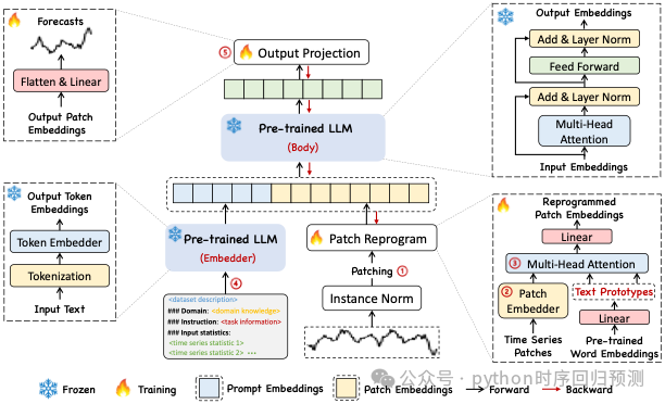
Time-LLM的核心理念是“重新编程”（reprogramming）：将时间序列数据转化为适合语言模型处理的形式，从而使其无需改变预训练的模型结构即可用于预测任务。该方法分为三个主要步骤：

1. 输入重构
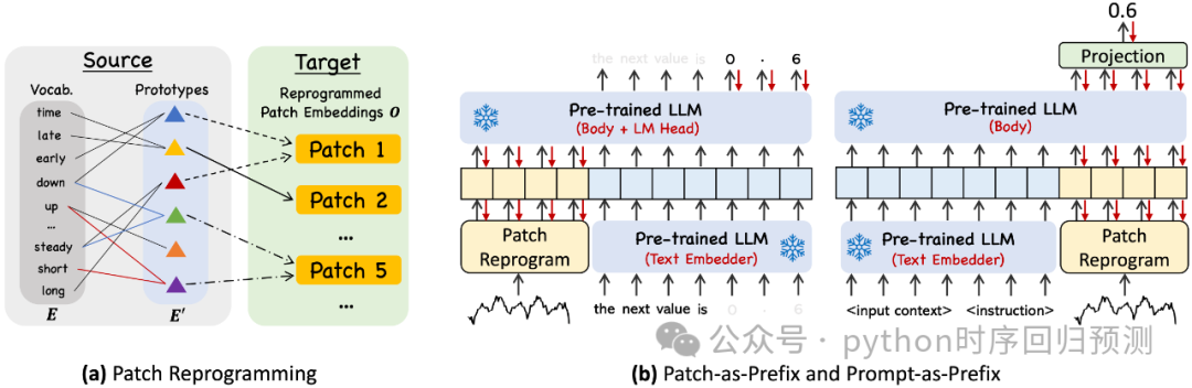
   时间序列数据被划分为若干小块（称为patch），每个小块通过线性变换生成嵌入表示。接着，这些嵌入被重新编程为“文本原型”（text prototypes）。这些原型以自然语言的形式表达时间序列的局部特征，帮助LLM理解数据模式。

2. 提示增强（Prompt-as-Prefix, PaP）
   为了更好地指导LLM处理时间序列数据，Time-LLM提出了“提示作为前缀”的策略。通过添加上下文信息、任务指令和输入统计信息（如趋势、延迟等），模型能更有效地推理并生成预测结果。

3. 输出投影
   LLM输出的高维嵌入被进一步线性映射为预测值。这种方式确保了整个框架的高效性，并保持LLM主体结构的冻结状态。

下面给出Time-LLM模型的部分代码，同样基于清华大学时间序列开源代码简化修改而来：

有想要其它相关模型的话可以咸鱼搜索“清朝简单的饮料”、“安仁坊天蝎座果”和“黉门街打球的生姜”，除这三个号外其它均为我的二次销售盗版（有些盗版连文案都不改一下直接复制我的就离谱），出了问题无法保障！！！此外csdn上也有较多我的盗版模型！！！！我的模型均使用焦作市的空气质量数据！！！注意甄别！！！！！老版本模型可能存在些许问题！！！！！还有最新的XLSTM、KAN-LSTM、TimesNet等等模型。也会陆续更新模型，欢迎关注！！！！！！​​​​​​

import numpy as np import torch  import torch.nn as nn from torch import optimfrom torch.utils.data import DataLoader, Dataset  import matplotlib.pyplot as plt import warnings  import pandas as pd  from sklearn.preprocessing import StandardScaler  from sklearn.metrics import mean_squared_error, mean_absolute_error, r2_score, mean_absolute_percentage_error  import math  from models import Time_LLMimport timefrom tqdm import tqdm warnings.filterwarnings('ignore') device = torch.device("cuda" if torch.cuda.is_available() else "cpu")df_raw = pd.read_excel('多变量.xlsx')target = 'canopy' col_ = df_raw.pop(target)df_raw.insert(1, target, col_)# 参数定义seq_len = 96  label_len = 24pred_len = 1  batch_size = 32epochs = 5scaler = StandardScaler()num_train = int(len(df_raw) * 0.7)num_test = int(len(df_raw) * 0.2)num_vali = len(df_raw) - num_train - num_testtrain_data = df_raw[:num_train]vali_data = df_raw[num_train:num_train + num_vali]test_data = df_raw[num_train + num_vali:]train_dataset = MyDataset(train_x, train_y, train_stamp)vali_dataset = MyDataset(vali_x, vali_y, vali_stamp)test_dataset = MyDataset(test_x, test_y, test_stamp)train_loader = DataLoader(train_dataset, batch_size=batch_size, shuffle=True, drop_last=True)vali_loader = DataLoader(vali_dataset, batch_size=batch_size, shuffle=False, drop_last=True)test_loader = DataLoader(test_dataset, batch_size=batch_size, shuffle=False, drop_last=True)
model = Time_LLM(    task_name='long_term_forecast',    seq_len=seq_len,    label_len=label_len,    pred_len=pred_len,    d_ff=512,    patch_len=16,    stride=8,    llm_model="GPT2",#'LLAMA' 'BERT' "GPT2"    llm_layers=2,    dropout=0.1,    enc_in=10,    prompt_domain=False,    content=None,    n_heads=8,).to(device)optimizer = optim.Adam(model.parameters(), lr=0.0001)criterion = nn.MSELoss()def vali(model, vali_loader, criterion, device, pred_len, label_len, output_attention=False):    total_loss = []    model.eval()    with torch.no_grad():        for batch_x, batch_y, batch_x_mark, batch_y_mark in vali_loader:            batch_x, batch_y, batch_x_mark, batch_y_mark = prepare_batch(batch_x, batch_y, batch_x_mark, batch_y_mark, device)            dec_inp = prepare_decoder_input(batch_y, pred_len, label_len, device)            outputs = get_model_outputs(model, batch_x, batch_x_mark, dec_inp, batch_y_mark, output_attention)            loss = criterion(outputs.cpu(), batch_y[:, -pred_len:, -1:].cpu())            total_loss.append(loss.item())        model.train()    return np.average(total_loss)for epoch in range(epochs):    train_loss = []    model.train()    for batch_x, batch_y, batch_x_mark, batch_y_mark in train_loader:        optimizer.zero_grad()        batch_x, batch_y, batch_x_mark, batch_y_mark = prepare_batch(batch_x, batch_y, batch_x_mark, batch_y_mark, device)        dec_inp = prepare_decoder_input(batch_y, pred_len, label_len, device)        outputs = get_model_outputs(model, batch_x, batch_x_mark, dec_inp, batch_y_mark, output_attention=False)        loss = criterion(outputs, batch_y[:, -pred_len:, -1:])        train_loss.append(loss.item())        loss.backward()        optimizer.step()    train_loss = np.average(train_loss)    vali_loss = vali(model, vali_loader, criterion, device, pred_len, label_len, output_attention=False)    test_loss = vali(model, test_loader, criterion, device, pred_len, label_len, output_attention=False)    print(f"Epoch: {epoch + 1}, Steps: {len(train_loader)} | Train Loss: {train_loss:.7f} Vali Loss: {vali_loss:.7f} Test Loss: {test_loss:.7f}")preds, trues = [], []model.eval()with torch.no_grad():    for batch_x, batch_y, batch_x_mark, batch_y_mark in test_loader:        batch_x, batch_y, batch_x_mark, batch_y_mark = prepare_batch(batch_x, batch_y, batch_x_mark, batch_y_mark, device)        dec_inp = prepare_decoder_input(batch_y, pred_len, label_len, device)        outputs = get_model_outputs(model, batch_x, batch_x_mark, dec_inp, batch_y_mark, output_attention=False)        preds.append(outputs[:, -pred_len:, :].cpu().numpy())        trues.append(batch_y[:, -pred_len:, :].cpu().numpy())preds, trues = np.concatenate(preds, axis=0), np.concatenate(trues, axis=0)plt.rcParams['font.sans-serif'] = ['SimHei'] plt.figure(figsize=(12, 4), dpi=600)plt.plot(trues[:, pred_len-1, 0], label='真实值', color='blue')for i in range(pred_len):    plt.plot(preds[:, i, 0], label=f'Step {i+1} Prediction')plt.title('真实值 vs 预测值')plt.xlabel('样本序号')plt.ylabel('目标值')plt.legend()plt.show()

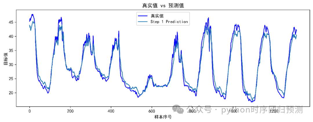
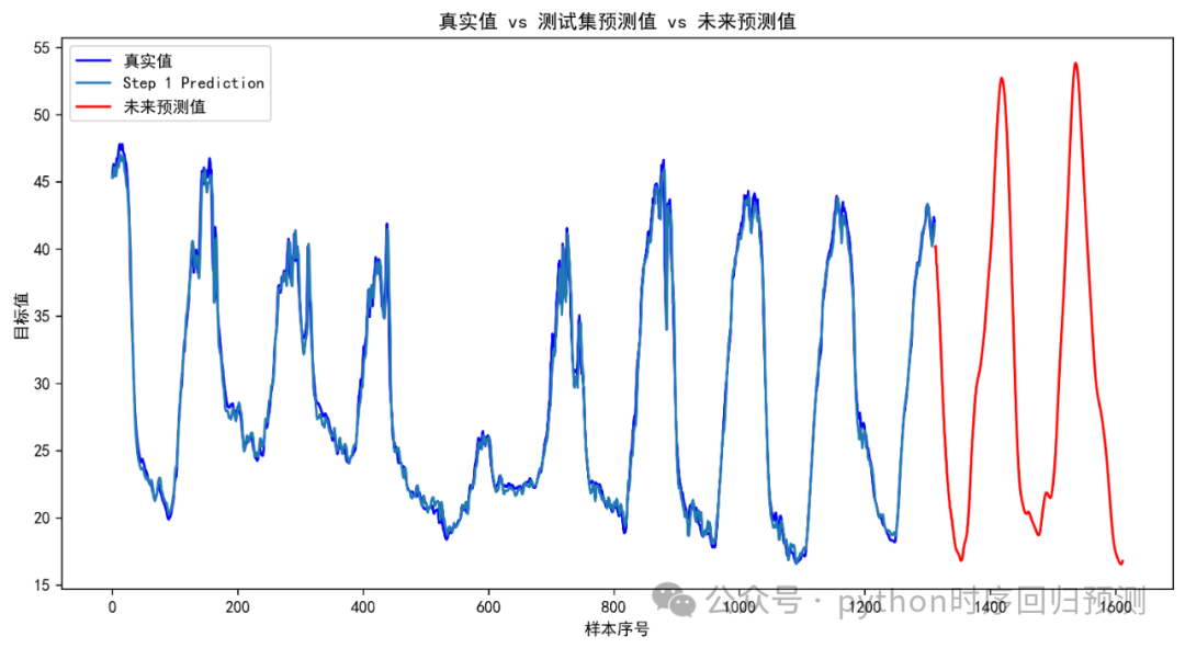
从本人实际运行来看，这个模型比较吃配置，以我上面给出的部分代码参数设置（推荐使用GPT2，会快一点并且不用搞其它东西）为例，运行7000多条的数据，迭代一次需要10分钟左右（本人笔记本电脑13900HX+4060），内存吃了17G多，专用显存和共享显存一共吃了18G多。因此需要该模型的同学可以自行对比一下自己的电脑配置和数据大小，也可以租个服务器跑。预测效果也在水准之内，如下图所示：

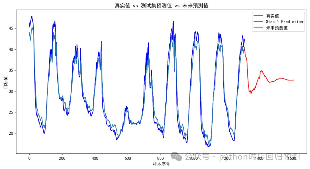
对未来300个值的预测效果如下：

此外上一篇文章的TimeMixer模型对未来值的预测效果如下：

模型原论文可以通过下面链接下载：https://openreview.net/pdf?id=Unb5CVPtae