


零基础学习深度学习
The ability to learn from experience and perform better when confronted with similar challenges is the trait of every intelligent person. Depending on where we are in our lives, what decides how far we go, is our ability and appetite to use the knowledge gained over a period of time. Artificial Intelligence, which is now considered to be the new “Electricity” operates on very similar principles. Rarely do we see an Artificial Neural Network (ANN) starting with 100% accuracy. The foundations of any ANN architecture starts with the premise that, the model needs to go through multiple iterations making allowance for mistakes, learn from mistakes and achieve salvation or saturation when it has learnt enough, thereby producing results equal to or similar to reality.
每个经验丰富的人的特征是,能够从经验中学习并在遇到类似挑战时表现更好。 根据我们生活中的位置,决定我们走多远的是,我们使用一段时间内获得的知识的能力和胃口。 如今被视为新的“电力”的人工智能以非常相似的原理运行。 我们很少看到以100%的准确性开头的人工神经网络(ANN)。 任何ANN架构的基础都以这样一个前提为出发点:该模型需要经历多次迭代,以留出错误的余地,从错误中吸取教训,并在充分学习后实现救赎或饱和,从而产生与现实相等或相似的结果。
The picture below gives us a brief idea of how an ANN looks like.
下图为我们简要介绍了人工神经网络的外观。

We see three layers of circles — Input, Hidden and Output — differentiated by their colors. Each of these circles are called as neurons and are seen to be interconnected. Hence the name neural network (or ANN). The first layer constitutes the input variables and has number of neurons equal to the number of input variables we may have. The last layer constitutes the representation of the number of categories/levels in the output variable, and hence called as output layer. The layer in the middle is where all the calculation happens. If we have multiple hidden layers, we call it a deep learning model. We generally do not have any control on the input or output layers as the inputs and outputs are predetermined by the problem we chose to solve. However we always have the ability to design the hidden layers (i.e. number hidden layers and number of neurons in each hidden layer) in such a way that, it gives us the best output.
我们看到三层圆圈-输入,隐藏和输出-通过它们的颜色来区分。 这些圆中的每个圆都称为神经元,并且被视为相互连接的。 因此,名称神经网络(或ANN)。 第一层构成输入变量,并且神经元数量等于我们可能具有的输入变量数量。 最后一层构成输出变量中类别/级别数量的表示,因此称为输出层。 中间的层是所有计算发生的地方。 如果我们有多个隐藏层,我们称之为深度学习模型。 我们通常对输入或输出层没有任何控制,因为输入和输出是由我们选择要解决的问题预先确定的。 但是,我们始终能够以这样的方式设计隐藏层(即,隐藏层的数量以及每个隐藏层中神经元的数量),从而为我们提供最佳输出。
My motivation in this article is to take you through what ANN is and how it achieves human like performance in many scenarios. The topics that will be covered are given below
在本文中,我的动机是带您了解什么是人工神经网络以及它在许多情况下如何实现类似于人类的性能。 下面列出了将要涉及的主题
Supervised Learning - Pathway to Nirvana
监督学习- 涅Ni之路
Deep Learning - A type of Supervised Learning Process
深度学习- 一种监督学习过程
Loss Function - Cycle of Karma, Samsara and Moksha
损失函数- 因果报应,轮回和莫沙的循环
Gears & Engine of Neural Network - Samagri, Upakarna and Zastra
神经网络的齿轮和引擎-Samagri,Upakarna和Zastra
Forward Propagation - Sequence of steps towards the destination
正向传播- 到达目的地的步骤顺序
Back Propagation - Calibration to reach the correct destination
反向传播- 校准以到达正确的目的地
Supervised Learning — Pathway to Nirvana
监督学习—通往涅Ni的途径
Supervised Learning is a Machine Learning (ML) task where a function is created that maps the relationship between input and output variables as it gets exposed to a large number of examples of input-output pair. The mapping is at two levels
监督学习是一种机器学习(ML)任务,其中创建了一个函数,当该函数暴露于大量输入/输出对示例时,该函数将映射输入和输出变量之间的关系。 映射分为两个级别
- relationship amongst the input variables 输入变量之间的关系
- relationship of the input variables as a whole with the output variable 输入变量作为整体与输出变量的关系
The function gets created as it gets exposed to many input-output pairs which essentially is the learning process. Thus the function produces an estimated output which is then compared with the actual output. This comparison for every input-output pair with the estimated output generates a feedback for the function until it figures out the exact rules for getting the accurate output. Hence the name supervised learning.
该函数是在暴露给许多输入/输出对时创建的,这实际上是学习过程。 因此,该函数会产生一个估计的输出,然后将其与实际输出进行比较。 每个输入-输出对与估计输出的比较都会对该函数产生反馈,直到它找出获取准确输出的确切规则。 因此,名称监督学习。
The diagram below will help in illustrating the concept even further
下图将有助于进一步说明该概念

As we can see above, the Supervised ML system constitutes the Model, the Optimization algorithm and the Loss function. The supervised learning system is fed with both the input variable x and the output y. The Model maps the function f(x) and predicts the output (=f(x)). The loss function compares y (actual output) and f(x) i.e the estimated/predicted output. If there is any difference, a signal (indicating the difference) is fed to the optimization algorithm as a feedback that updates/adjusts the parameters in the model to improve the results generated by the function i.e. f(x). This process continues until there is very little difference between the predicted output i.e. f(x) and the desired output i.e. y.
正如我们在上面看到的那样,监督式机器学习系统由模型,优化算法和损失函数组成。 有监督的学习系统既可以输入变量x也可以输出变量y。 模型映射函数f(x)并预测输出(= f(x))。 损失函数将y(实际输出)与f(x)(即估计/预测输出)进行比较。 如果存在任何差异,则将信号(指示差异)作为反馈反馈给优化算法,该反馈会更新/调整模型中的参数以改善函数(即f(x))生成的结果。 这个过程一直持续到预测输出即f(x)与期望输出即yy之间几乎没有差异为止。
The parameters essentially are the learnable objects in the machine learning algorithm that continue to be updated until there is very little difference between the actual and the predicted output (i.e. f(x)). The hyper-parameters are design elements in the machine learning algorithm that we decide and experiment to get better results. They are not learnable. For example, weights in an ANN are learnable parameters which gets updated after every iteration. Whereas number of layers or neurons in each layer are design elements in a deep learning network which are not learnable. The developer experiments and decides the best hyper-parameters, based on results.
这些参数本质上是机器学习算法中的可学习对象,这些对象将继续更新,直到实际输出和预测输出之间的差异很小(即f(x))。 超参数是我们决定并进行实验以获得更好结果的机器学习算法中的设计元素。 他们是无法学习的。 例如,ANN中的权重是可学习的参数,每次迭代后都会更新。 而每层中的层数或神经元是深度学习网络中不可学习的设计元素。 开发人员根据结果进行实验并确定最佳的超参数。
深度学习-一种监督学习过程 (Deep Learning - A type of Supervised Learning Process)
Deep Learning (DL) is a special branch of Machine Learning as can be seen in the pictorial representation of the relationship between AI (Artificial Intelligence), ML (Machine Learning) and DL (Deep Learning).
深度学习(DL)是机器学习的一个特殊分支,从AI(人工智能),ML(机器学习)和DL(深度学习)之间的关系的图示中可以看出。

The fundamentals of Supervised Learning, which is the foundation of any Machine Learning framework applies to DL as well. The major difference is primarily in the architecture.
监督学习的基础是任何机器学习框架的基础,也适用于DL。 主要区别主要在于体系结构。
The fundamental difference at a structural level is the ability of deep learning models to learn the features and feature of features from base data. Traditional ML algorithms require the input data to be pre-processed including feature engineering — extraction, generation and transformation wherever applicable. The representation below will help with illustration of the difference.
在结构级别上的根本区别是深度学习模型从基础数据中学习特征和特征的能力。 传统的机器学习算法要求对输入数据进行预处理,包括特征工程-提取,生成和转换(如果适用)。 下面的表示形式将有助于说明差异。

DL is achieving exemplary results in areas where human intuition would have played a big role. Traditional ML algorithms were not able to achieve results like the DL algorithms are doing on perceptual problems such as hearing and seeing.
DL在人类直觉将发挥重要作用的领域中取得了可喜的成绩。 传统的ML算法无法像DL算法那样在听觉和视力等感知问题上取得成果。
A few examples of where deep learning has achieved breakthroughs, all in historically difficult areas of machine learning are given below:
下面提供了一些示例说明了深度学习在机器学习的历来困难领域取得了突破的情况:
- Near human level image classification 近人图像分类
- Near human level speech recognition 近人语音识别
- Ability to answer natural language questions 回答自然语言问题的能力
- Improved ad targeting, as used by Google, Baidu, and Bing 改进了广告定位,如Google,百度和Bing所使用的
- Digital assistants such as Google Now and Amazon Alexa Google即时和亚马逊Alexa等数字助理
One may ask what is the difference between ANN and DL. The name Artificial Neural Network is inspired from a rough comparison of it’s architecture with human brain. Although some of the central concepts in ANNs were developed in part by drawing inspiration from our understanding of the brain, ANN models are not models of the brain. In reality, there is no great similarity between an ANN and it’s method of operation with human brain, neurons, synapses and it’s modus operandi. However the fact that the ANN is a consolidation of one or more layers of neurons, that help in solving perceptual problems - which is based human intuition, the name goes well.
可能有人会问ANN和DL有什么区别。 人工神经网络这个名称的灵感来自它与人脑的粗略比较。 尽管人工神经网络的一些核心概念部分是通过我们对大脑的了解获得灵感而开发的,但人工神经网络模型并不是大脑的模型。 实际上,人工神经网络与它与人脑,神经元,突触及其操作方式的操作方法之间并没有很大相似之处。 然而,ANN是一层或多层神经元的合并,这有助于解决感知问题,这是基于人类直觉的事实,这个名称很合适。
ANN essentially is a structure consisting of multiple layers of processing units (i.e. neurons) that take input data and process it through successive layers to derive meaningful representations. The word deep in Deep Learning stands for this idea of successive layers of representation. How many layers contribute to a model of the data is called the depth of the model.
人工神经网络本质上是由多层处理单元(即神经元)组成的结构,这些处理单元获取输入数据并通过连续的层对其进行处理以得出有意义的表示。 深度学习中的“深层”一词代表连续表示层的想法。 数据模型中有多少层被称为模型深度。
Below diagram illustrates the structure better as we have a simple ANN with only one hidden layer and a DL Neural Network (DNN) with multiple hidden layers. Thus DL or DLNN is an ANN with multiple hidden layers.
下图显示了更好的结构,因为我们有一个仅具有一个隐藏层的简单ANN和一个具有多个隐藏层的DL神经网络(DNN)。 因此,DL或DLNN是具有多个隐藏层的ANN。

The learning process in DL can be explained as below.
DL中的学习过程可以解释如下。

The fundamentals of supervised learning explained in the first section are still the same. The only difference here would be the structural difference between a DL model from traditional ML models and how the information flows both from input to output (forward propagation) and from output to weights (backward propagation). We will see these in more detail in the forthcoming sections.
第一部分中解释的监督学习的基础仍然相同。 唯一的区别是,传统ML模型的DL模型与信息如何从输入流向输出(正向传播)以及从输出流向权重(向后传播)之间的结构差异。 我们将在接下来的部分中详细介绍这些内容。
Loss Function — Cycle of Karma, Samsara and Moksha
损失函数—因果报应,轮回和莫沙的循环
From figure 1 and figure 5, we get a fair understanding of the criticality of the loss functions. The role of loss function is pivotal in ensuring that the output from the Supervised ML system is constantly nudged towards the actual values. ML/DL is said to mimic human behavior not just because it gives us near human like intuitive result/accuracy but also because it’s method to achieve the result is similar to human philosophy of learning. Humans learn from their mistakes and leverage experience to make wise decisions in various stages of life. Similarly, the DL(and ML)algorithms make room for mistakes in the initial iterations ,which are represented by loss scores or signals, calculated by the loss functions. These loss scores are fed back to the algorithms to update the weights in such a way that the next predicted output gets closer to the actual value. Thus, it is a cyclical process, where each iteration is like a cycle and the cycle continues till the loss is minimized. Very similar to Hindu philosophy of Karma, Samsara and Moksha.
从图1和图5中,我们对损失函数的重要性有了一个很好的了解。 损失函数的作用对于确保将监督ML系统的输出不断推向实际值至关重要。 据说ML / DL模仿人类行为,不仅是因为它使我们像直观的结果/准确性一样接近人类,而且因为达到结果的方法类似于人类的学习哲学。 人类从错误中学习并利用经验在人生的各个阶段做出明智的决定。 类似地,DL(和ML)算法为初始迭代中的错误留出了空间,这些错误由损失分数或信号(由损失函数计算)表示。 这些损耗分数将反馈给算法以更新权重,以使下一个预测输出更接近于实际值。 因此,这是一个循环过程,其中每次迭代都像一个循环,并且该循环一直持续到损失最小为止。 非常类似于印度教的业力,轮回和莫克沙哲学。
Considering the importance of loss functions, it is critical to know how it operates and hence choose the appropriate one to achieve Moksha i.e. zero loss. Our goal is to minimize the loss i.e. find the point where the loss is zero. For this we need to choose a loss function which can aid us in finding a minimum. Thus we need a loss function whose surface is convex in shape. If we choose a function, which is concave in nature, we may not have a minimum (also called as minima) and hence we will be derailed from our goal. The figure below will illustrate the point further.
考虑到损失函数的重要性,至关重要的是要了解其运行方式,并因此选择合适的函数来实现Moksha,即零损失。 我们的目标是使损失最小化,即找到损失为零的点。 为此,我们需要选择一个损失函数,该函数可以帮助我们找到最小值。 因此,我们需要一个损失函数,其表面为凸形。 如果我们选择的函数本质上是凹形的,则我们可能没有最小值(也称为最小值),因此我们会偏离目标。 下图将进一步说明这一点。

We see two functions i.e. f(x) and q(x) above and their respective graphical representation. The function f(x) is convex in nature and has a minimum value i.e. the vertex with co-ordinates (-5/4, -1/4). On the other hand, function q(x) has a concave shape and we can only find a maxima here. We cannot find the minimum value on it’s surface. So while we are building our ML or DL network, we need to choose a loss function which has a shape like f(x) i.e. convex in nature. The algorithm’s goal in that case would be to iterate until the weights are adjusted such that we move along the surface of f(x) and reach the vertex (-5/4, -1/4) i.e. the global minima. The mechanics of how we move from any point on the loss function to the minima is explained by a concept called gradient descent (to be covered in the next section). Since choice of a loss function is critical, the two most widely used loss functions are
我们看到上面的两个函数,即f(x)和q(x)以及它们各自的图形表示。 函数f(x)本质上是凸的,并且具有最小值,即具有坐标(-5/4,-1/4)的顶点。 另一方面,函数q(x)具有凹形,我们在这里只能找到一个最大值。 我们无法在其表面上找到最小值。 因此,当我们构建ML或DL网络时,我们需要选择一个损失函数,其形状类似于f(x),即自然凸。 在这种情况下,算法的目标是迭代直到调整权重,使得我们沿着f(x)的表面移动并到达顶点(-5/4,-1/4),即全局最小值。 我们如何从损失函数的任意点移至最小值的机制由称为梯度下降的概念解释(将在下一节中介绍)。 由于损失函数的选择至关重要,因此使用最广泛的两个损失函数是
a. Mean Square Error for regression problems (the output is numeric in nature, for example prediction of price of a house)
一个。 回归问题的均方误差(输出本质上是数字的,例如,房屋价格的预测)
Formula: L= 1/2*(y-f(x))²
公式:L = 1/2 *(yf(x))²
b. Categorical Cross Entropy for classification problems (the output is categorical in nature, for example predicting whether a student will pass the exam or not)
b。 分类问题的分类交叉熵(输出本质上是分类的,例如预测学生是否会通过考试)
Formula: L =-[y*log(f(x))+(1-y)*log(1-f(x))]
公式:L =-[y * log(f(x))+(1-y)* log(1-f(x))]
Gears & Engine of Neural Network - Samagri, Upakarna and Zastra
神经网络的齿轮和引擎 -Samagri,Upakarna和Zastra
We have so far established two import factors to achieve the best results with a Deep Learning network. They are
到目前为止,我们已经建立了两个导入因素,以通过深度学习网络实现最佳结果。 他们是
- Loss function - Plays an extremely critical role in ensuring that the accuracy of the system is gradually optimized 损失功能-在确保逐步优化系统准确性方面发挥着至关重要的作用
- Minima - The optimization is achieved by locating the minima of the loss function (which should be convex in shape) 最小值-通过找到损失函数的最小值(形状应为凸形)来实现优化
The key to reach the minima of a loss function is the ability to know which direction we should move, at any point on the surface of a loss function, and by how much, so that we can reach the minima in as less number of iterations as possible. This requirement introduces us to a few more concepts which can be considered to be the tools, nuts, bolts and gears of an ANN. They are as given below
达到损失函数最小值的关键是能够知道我们应该在损失函数表面上的任意点移动哪个方向,以及移动多少,以便我们能够以更少的迭代次数达到最小值。尽可能。 这项要求向我们介绍了更多概念,可以将它们视为ANN的工具,螺母,螺栓和齿轮。 它们如下
- Scalar, Vector, Function 标量,向量,函数
- Derivative of a function 函数的导数
- Chain rule of differentiation 差异化的连锁法则
- Double Derivative 双导数
- Hessian and Jacobian 黑森州和雅各布主义
- Gradient ascent and descent 梯度上升和下降
The above are important components of linear algebra and I am assuming familiarity of the reader with them. For refresher, the reader can explore freely available material on these topics in internet. Going through each of them in-depth is beyond the scope of this article. We will however focus on gradient descent which can be considered to be the engine of DL. The rest of the above bullets are like tools that help in facilitating smooth functioning of the engine. Gradient descent is essentially the technique that helps ANN reach the minima of a loss function. Let’s see how.
以上是线性代数的重要组成部分,我假设读者熟悉它们。 作为复习,读者可以在Internet上免费浏览有关这些主题的材料。 对它们的深入研究超出了本文的范围。 但是,我们将专注于可以认为是DL引擎的梯度下降。 上面的其余项目符号就像工具,有助于促进引擎的平稳运行。 梯度下降本质上是帮助ANN达到损失函数最小值的技术。 让我们看看如何。
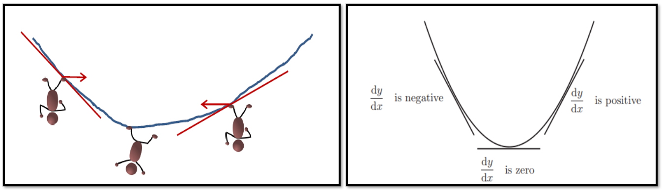
For being able to understand gradient descent, let’s first understand gradient ascent. If we are trying to climb a mountain, irrespective of where we are at, as long as we can gauge the slope, we will know which direction to move towards so that we reach the peak i.e. the maxima. For simplicity of understanding, let’s assume that the shape of the mountain is represented by function y=f(x), where x is the horizontal axis. Slope is defined as the change in the value of the function for a small change in x. Mathematically, this would translate to dy/dx which is the derivative of the function, f(x). Geometrically slope is always tangent to the surface. See below for illustration.
为了能够理解梯度下降,让我们首先了解梯度上升。 如果我们试图爬山,无论我们身在何处,只要可以测量坡度,我们都将知道向哪个方向移动,以便到达山峰即最大值。 为了简化理解,我们假设山的形状由函数y = f(x)表示,其中x是水平轴。 斜率定义为x值有微小变化时函数值的变化。 从数学上讲,这将转换为dy / dx,它是函数f(x)的导数。 几何坡度始终与曲面相切。 请参阅下面的插图。

We see the mountain and a person trying to climb to the peak from either direction in the left picture of figure 7 above. The picture on the right tells us the direction of slope of the mountain when the man would be trying to climb from either direction. Notice that the value of the slope at the peak is zero. This is so because for a small change in x, there is no change in vertical direction, i.e. y. So change in y is zero for a very small change in x. Hence dy/dx = 0. Assuming that our mountain is represented by a smooth concave shaped parabola as shown above, we will have only one possible peak which can be reached at by moving in the direction of where the slope of the function is zero. With that established, if we are on the left hand side of the mountain, the slope of the mountain is positive (as the tangent is inclined towards the positive direction of x). Hence we need to move towards right i.e. in the direction of the slope to reach the maxima. Similarly, if we are on the right hand side of the mountain, the slope is negative (as the tangent is inclined towards the negative direction of x). Hence we need to move towards left i.e. in the direction of the slope to reach the maxima.
在上图7的左图中,我们看到了一座山和一个试图从任一方向爬到山顶的人。 右图告诉我们该人试图从任一方向爬山时的山坡方向。 请注意,峰值处的斜率值为零。 之所以如此,是因为对于x的很小变化,垂直方向没有变化,即y因此,对于x的很小变化,y的变化为零。 因此dy / dx =0。 假设我们的山峰由上图所示的光滑凹形抛物线表示,则在函数斜率为零的方向上移动时,我们将只有一个可能的峰值。 建立好后,如果我们在山的左侧,则山的斜率为正(因为切线向x的正方向倾斜)。 因此,我们需要向右移动,即朝斜坡的方向移动,以达到最大值。 同样,如果我们在山的右侧,则坡度为负(因为切线向x的负方向倾斜)。 因此,我们需要向左移动,即朝坡度方向移动,以达到最大值。
Thus in summary, if we know that our function is concave shaped and hence has a maxima, we can reach the peak by leveraging the slope of the function at any point on the surface of the function.
因此,总而言之,如果我们知道函数是凹形的并因此具有最大值,则可以通过利用函数表面上任意点的函数斜率来达到峰值。
Similarly, lets indulge in the figure below, to reach the minima. The function f(x) could be our loss function and we are interested to get to the minima for reasons explained in earlier sections of the article. The loss function as you can see is an inverted mountain (inversion of the figure 7) and is convex in nature.
同样,让我们沉迷于下图中,以达到最小值 。 函数f(x)可能是我们的损失函数,由于本文前面各节中说明的原因,我们有兴趣获得最小值。 如您所见,损失函数是一个颠倒的山脉(图7的颠倒),本质上是凸的。
The picture on the right tells us the direction of slope of the loss function when the man would be trying to reach the lowest point of the surface from either direction. Notice that the value of the slope at the lowest point i.e. minima is zero. This is so because for a small change in x, there is no change in the vertical direction, i.e. y. So, change in y is zero for a very small change in x. Hence dy/dx = 0. Assuming that our loss function is represented by a smooth convex shaped parabola as shown above, we will have only one possible minima which can be reached at by moving in the direction of where the slope of the function is zero. With that established, if we are on the left hand side of the surface, the slope of the mountain is negative (as the tangent is inclined towards the negative direction of x). Hence we need to move towards right i.e. in the opposite direction of the slope to reach the minima. Similarly, if we are on the right hand side of the surface, the slope is positive (as the tangent is inclined towards the positive direction of x). Hence we need to move towards left i.e. in the opposite direction of the slope to reach the maxima.
右图告诉我们当人试图从任一方向到达表面的最低点时,损失函数的斜率方向。 请注意,最低点处的斜率值(即最小值)为零。 之所以如此,是因为对于x的微小变化,垂直方向没有变化,即y。因此,对于x的很小变化,y的变化为零。 因此dy / dx =0。 假设我们的损失函数由如上所示的光滑凸形抛物线表示,则在函数斜率为零的方向上移动时,我们将只有一个可能的最小值。 。 建立后,如果我们在表面的左侧,则山的坡度为负(因为切线向x的负方向倾斜)。 因此,我们需要向右移动,即在与坡度相反的方向上移动,以达到最小值。 同样,如果我们在曲面的右侧,则斜率是正的(因为切线朝着x的正方向倾斜)。 因此,我们需要向左移动,即在与坡度相反的方向上移动以达到最大值。
Thus in summary, if we know that our function is convex shaped and hence has an unique minima, we can reach the bottom/minima by leveraging the slope of the function at any point on the surface of the function.
因此,总而言之,如果我们知道我们的函数是凸形的并因此具有唯一的最小值,则可以通过利用函数表面上任意点的函数斜率来达到底部/最小值。
So, in the context of the topic, we can conclude that, at any point on the surface of a function f(x), we always need to move towards the point where the slope of the surface is zero. However in the above examples we knew that the surface is concave or convex which helped us with the knowledge that we are approaching either the maxima or the minima respectively without any doubt. What if we do not have prior knowledge of the shape of the surface? How would we know that our movement is taking us towards the maxima or minima?
因此,在本主题的上下文中,我们可以得出结论,在函数f(x)的曲面上的任何点,我们总是需要朝曲面的斜率为零的点移动。 但是,在以上示例中,我们知道该表面是凹面还是凸面,这无疑使我们了解到我们正分别接近最大值或最小值。 如果我们不了解表面形状怎么办? 我们怎么知道我们的运动正在把我们带向最大或最小?
This is where the concept of double derivative comes to our rescue. See the picture below for better illustration.
这就是双导数概念为我们解救的地方。 请参阅下面的图片以获得更好的插图。

If f(x) is our function, slope of the function at either the minima or maxima on the surface is zero i.e. 2ax+b=0.
如果f(x)是我们的函数,则函数在表面上的最小值或最大值处的斜率为零,即2ax + b = 0。
However, if we calculate the derivative of the slope, we get a constant i.e. 2a. If the value of 2a is positive, we know that our function is convex, and we need to move in a direction opposite to the slope to reach the minima. The left section of the figure 9 illustrates the same.
但是,如果我们计算斜率的导数,我们将得到一个常数,即2a。 如果2a的值为正,则表明我们的函数是凸的,并且需要沿与斜率相反的方向移动以达到最小值。 图9的左部分示出了相同的内容。
Similarly, if the value of 2a is negative, we know that our function is concave, and we need to move in the direction of the slope to reach the maxima. The right section of the figure 9 illustrates the same.
类似地,如果2a的值为负,则我们知道函数是凹面的,我们需要沿倾斜方向移动以达到最大值。 图9的右半部分对此进行了说明。
Thus in summary, if we have a loss function which is differentiable and convex in nature, we can leverage derivative and double derivative to reach the minima. Subsequently we can optimize our supervised learning model by adjusting our weights to improve accuracy.
因此,总而言之,如果我们具有本质上可微且凸的损失函数,则可以利用导数和双导数来达到最小值。 随后,我们可以通过调整权重以提高准确性来优化监督学习模型。
At every point i.e. in every iteration, the DL network calculates the estimated or predicted output (i.e. f(x) in the context of figure 1) and the slope of the loss function w.r.t weights, which is called as the gradient of the loss w.r.t weights. Then the network takes a step towards the negative gradient of the loss, where the minima is identified through iterations. The new concept now is the step size which decides how fast the algorithm optimizes.
在每个点,即每次迭代中,DL网络都会计算估计或预测的输出(即在图1中为f(x))和损失函数wrt权重的斜率,这称为损失wrt的梯度重量。 然后,网络朝着损耗的负梯度迈出了一步,其中通过迭代确定了最小值。 现在,新概念是步长,它决定了算法优化的速度。

Step size is a hyper-parameter and is not a learnable parameter in DL.
步长是一个超参数,不是DL中可学习的参数。
Forward Propagation — Sequence of steps towards the destination
正向传播-到达目的地的步骤顺序
Right then, we are now at the business end. So far we have focused a lot on how the DL system learns. The DL system leverages a loss function as discussed in the previous section to send signals back (as feedback)to the hidden layers for the purposes of learning. This process of sending feedback back to the hidden layers is called as back propagation which will be covered in the next section.
那时,我们现在处于业务端。 到目前为止,我们已经集中精力研究DL系统的学习方式。 DL系统利用上一节中讨论的损失功能将信号发送(作为反馈)给隐藏层,以供学习之用。 将反馈发送回隐藏层的过程称为反向传播,将在下一部分中介绍。
But before that let’s understand the flow of information from the input to the output layer. The information flows from the input layer to the output through the hidden layers helping with sequential feature learning. Let’s understand the math behind it. This process is called as forward propagation.
但是在此之前,让我们了解从输入到输出层的信息流。 信息从输入层通过隐藏层流向输出,有助于顺序特征学习。 让我们了解其背后的数学原理。 此过程称为正向传播。

The figure above represents a fully connected deep learning structure with two hidden layers. The picture on the right represents how the output from each input layer is calculated. It’s a two step process. First the weighted sum of all inputs is calculated which is a linear transformation of the input. The weighted sum is then fed to an activation function which acts like a gate as it decides whether the neuron is switched on or not. The below diagram will help in simplifying the calculation further.
上图表示具有两个隐藏层的完全连接的深度学习结构。 右图表示如何计算每个输入层的输出。 这是一个两步过程。 首先,计算所有输入的加权和,这是输入的线性变换。 然后将加权总和馈入激活函数,该函数在确定神经元是否打开时起着门的作用。 下图将有助于进一步简化计算。
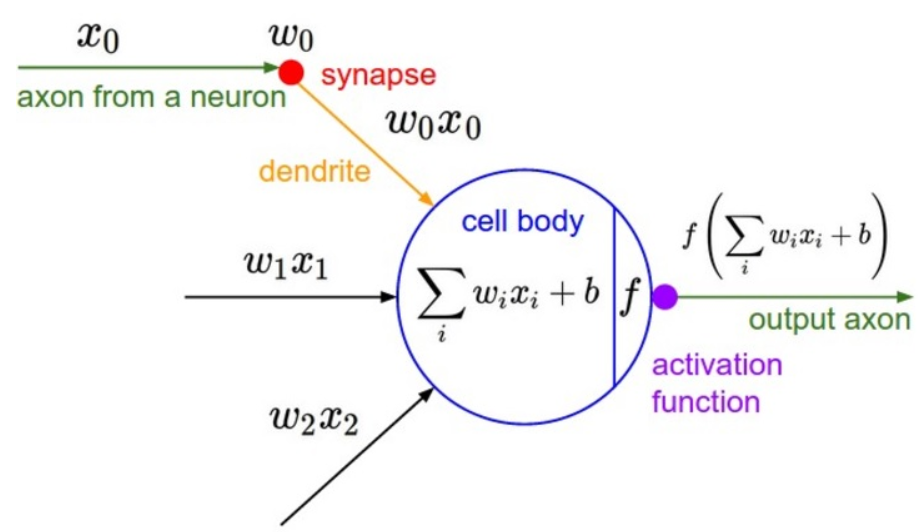
Here we see that there are three inputs represented by x1,x2 and x3. We have weights, w0, w1 and w2. The two step process as explained above results in weighted sum of the weights and inputs, followed by calculation from the activation function. If the output from the activation function is greater than 0, the neuron fires or stays inactive.
在这里,我们看到由x1,x2和x3表示的三个输入。 我们有权重w0,w1和w2。 如上所述的两步过程导致权重和输入的加权总和,然后根据激活函数进行计算。 如果激活函数的输出大于0,则神经元触发或保持不活动状态。
The simplified numerical or matrix calculation method for the output of a simple neural layer is illustrated below. Here we have four input variables and the output layer has three neurons. It’s a fully connected layer with all neurons in the input and output layer interconnected. The weights for these connections are color coded. The blue lines indicate connections between a1 and all inputs, the green between a2 and all inputs and likewise orange for a3. Each of these connections is represented by a weight - w1, w2, w3 and w4. See the first matrix in the below picture. These weights are the learnable parameters and the primary goal in DL (or in any ML) is to update these updates, through iterations, such that the predicted(or calculated) output equates the actual output.
下面说明了用于简单神经层输出的简化数值或矩阵计算方法。 这里我们有四个输入变量,输出层有三个神经元。 它是一个完全连接的层,输入和输出层中的所有神经元都相互连接。 这些连接的权重用颜色编码。 蓝线表示a1和所有输入之间的连接,绿色表示a2和所有输入之间的连接,同样表示a3的橙色。 这些连接中的每一个都由权重-w1,w2,w3和w4表示。 请参见下图的第一个矩阵。 这些权重是可学习的参数,DL(或任何ML)中的主要目标是通过迭代来更新这些更新,以使预测(或计算)的输出等于实际输出。

The activation function introduces non-linearity by converting the weighted sum of weights into a polynomial of higher degree, thereby allowing non-linear decision boundaries. The major advantage and reason for introducing non-linearity through activation function is to be able to create a decision boundary to separate classes which are linearly not separable. See below
激活函数通过将权重的加权和转换为更高次多项式来引入非线性,从而允许非线性决策边界。 通过激活函数引入非线性的主要优点和原因是能够创建决策边界以分离线性不可分离的类。 见下文

The picture on the left shows classifications with a linear separator. The separation is much better in the right hand side picture where we have a non-linear classifier. There are many types of activation functions, namely - sigmoid, tanh, step, relu and many versions of relu. I would not go into details of each of these as that would be become an article in itself. I may write another article explaining various activation functions and associated concepts. However, at this point, it is safe to say, relu seems to be most widely used as it helps seems to be improving the performance of ANNs more than other activation functions.
左图显示了带有线性分隔符的分类。 在具有非线性分类器的右侧图片中,分离效果更好。 激活函数有很多类型,即-Sigmoid,tanh,step,relu和relu的许多版本。 我不会详细介绍这些内容,因为它们本身将成为一篇文章。 我可能还会写另一篇文章,解释各种激活功能和相关概念。 但是,在这一点上,可以肯定地说,relu似乎得到了最广泛的应用,因为它似乎比其他激活功能更能改善ANN的性能。
If we simplify the figure 10 to what we see below in figure 11, the explanation for calculation of the output at each layer during forward propagation will become easier.
如果将图10简化为下面在图11中看到的内容,则在前向传播期间计算每一层的输出的解释将变得更加容易。


Back Propagation — Calibration to reach the correct destination
反向传播—校准以到达正确的目的地

Once we have the output, the most important step in deep learning to enable the algorithm to learn is to compare the output with the actual target variable. In the picture above, we see that being done by the Loss function L. The next step in the process is to find a way to send the signal (representing the loss) back to the hidden layers and update the weights such that, the loss reduces iteratively to it’s minima. So essentially, we are interested in finding the point on the loss surface, where the loss does not seem to change even when the weights are changing (in small amount). Technically we intend to find the point on the loss surface where it’s slope with respect to weights is equal to zero.
有了输出后,深度学习中使算法能够学习的最重要步骤是将输出与实际目标变量进行比较。 在上图中,我们看到通过损耗函数L完成。过程的下一步是找到一种方法,将信号(代表损耗)发送回隐藏层并更新权重,从而使损耗迭代地减少到最小值。 因此,从本质上讲,我们感兴趣的是找到损失表面上的一点,即使权重发生变化(少量),损失似乎也不会发生变化。 从技术上讲,我们打算在损失面上找到相对于权重的斜率等于零的点。

Keeping in mind the concept of gradient descent in the previous sections, and knowing that our loss function is convex in nature, the algorithm will continually take steps towards the minima i.e. we will keep moving in a direction opposite to the slope (or tangent) at any point until, the slope becomes zero.
牢记前面几节中的梯度下降的概念,并且知道我们的损失函数本质上是凸的,因此算法将不断朝着最小值迈进,即我们将继续沿与坡度(或切线)相反的方向移动直到斜率变为零为止。
The algorithm takes care of all the above calculations and it’s best to leave it to the machine as it has much higher computational competency. However the high level mathematical understanding of what goes under the hood is good to know for conceptual understanding. The below diagram helps us with it, where chain rule concept in derivatives is used to calculate the partial derivatives of loss with respect to the weights.
该算法负责上述所有计算,最好将其留给计算机,因为它具有更高的计算能力。 但是,对于概念上的了解,对于幕后的事物具有高水平的数学理解是很好的。 下图为我们提供了帮助,其中衍生工具中的链规则概念用于计算权重损失的偏导数。

In order to be be able to calculate slope of loss, L, with respect to weights in Layer 5, we require L to be differentiable by weights in Layer 5. However that is not the case. Hence the chain rule is invoked. See below
为了能够相对于第5层中的权重计算损耗的斜率L,我们要求L在第5层中的权重是可微的。但是,事实并非如此。 因此,调用链规则。 见下文
Once we have partial derivative of L with respect to W5, weights in Layer 5 can be updated to nudge the loss towards it’s minima. The next step is to be able to update weights in Layer 3 like in Layer 5.
一旦有了关于W5的L的偏导数,就可以更新第5层中的权重,以将损失推向最小值。 下一步是能够像在第5层中一样在第3层中更新权重。

The diagram above explains how the signal flows from loss function through to Layer 3. It can be seen how chain rule is utilized as was for updating weights in Layer 5.
上图说明了信号如何从损耗函数流到第3层。可以看出如何使用链规则来更新第5层中的权重。
The feedback from the Loss function to Layer 5 is
从损失功能到第5层的反馈是
The feedback from the Loss function to Layer 4 is
从损失功能到第4层的反馈是


The feedback from Loss Function to layer 3 is
从损失函数到第3层的反馈是

Thus for updating weights in Layer 3, the required calculation representing slope of Loss with respect to weights in Layer 3, is expressed as below
因此,为了更新第3层中的权重,表示所需损失的斜率相对于第3层中的权重的计算公式如下所示

The pictorial representation of backward propagation for updating weights in Layer 3 (and also Layer 5) is shown below
下图显示了用于在第3层(以及第5层)中更新权重的向后传播的图形表示形式

By following the same concepts the weights in Layer 1 also gets updated.
通过遵循相同的概念,第1层中的权重也会得到更新。
The cycle of forward propagation, backward propagation and weights update continues until the algorithm optimizes to arrive at the minimum value of loss achievable. At this point the best performance from the deep learning model is expected to be achieved.
继续向前传播,向后传播和权重更新的循环,直到算法进行优化以达到可实现的最小损失值为止。 在这一点上,有望实现深度学习模型的最佳性能。
Conclusion
结论
This article was aimed at introducing the fundamentals of Deep Learning to the reader. Artificial Intelligence has been in vogue for a while now, and Deep Learning has gained prominence in the last two decades. ANN (and DL) is not a new concept. It has gone through a few AI winters, in 1950s, 60s and a few more times until the turn of the century. It has been evolving and now producing results like never before. A key trigger for renewed interest in neural networks and learning was introduction of back-propagation algorithm that enabled practical training of multi-layer networks. Back propagation distributed the error term back up through the layers, by modifying the weights at each node. Additionally, the below factors have propelled interest and enabled success of ANNs (and DL)
本文旨在向读者介绍深度学习的基础知识。 人工智能已经流行了一段时间了,在过去的二十年中,深度学习已经变得越来越重要。 ANN(和DL)不是一个新概念。 它经历了1950年代,60年代的几个AI冬季,直到世纪之交。 它一直在发展,现在产生前所未有的结果。 对神经网络和学习重新产生兴趣的一个关键触发因素是反向传播算法的引入,该算法使得能够对多层网络进行实际训练。 反向传播通过修改每个节点的权重,将误差项分配到各层。 此外,以下因素引起了人们的兴趣,并使得ANN(和DL)取得了成功
- Evolution of the world to huge computational capabilities 世界进化到强大的计算能力
- Robust data collection methods and 强大的数据收集方法和
- Access to humongous data through improved storage facilities (like cloud) 通过改进的存储设施(例如云)访问庞大的数据
This is the first of a series of articles to come, where we will cover how DL is helping us achieve great results. This article focused on the foundations which will be followed by application of the concepts learnt in solving problems. We will see how DL is used in Computer Vision, NLP etc. in the forthcoming articles.
这是系列文章中的第一篇,我们将介绍DL如何帮助我们取得巨大的成就。 本文重点介绍了基础,随后将应用在解决问题中学到的概念。 在接下来的文章中,我们将了解如何在计算机视觉,NLP等中使用DL。
翻译自: https://medium.com/analytics-vidhya/foundations-of-deep-learning-7832d4fe5458
零基础学习深度学习


 4452
4452

 被折叠的 条评论
为什么被折叠?
被折叠的 条评论
为什么被折叠?
 到【灌水乐园】发言


