元学习迁移学习_元学习就是您所需要的

最新推荐文章于 2024-04-21 12:31:57 发布

weixin_26726011

最新推荐文章于 2024-04-21 12:31:57 发布

阅读量1.9k

点赞数

文章标签： python 人工智能机器学习编程语言深度学习

原文链接：https://medium.com/cracking-the-data-science-interview/meta-learning-is-all-you-need-3bd0bafdf289

版权

元学习迁移学习

Update: This post is part of a blog series on Meta-Learning that I’m working on. Check out part 1 and part 2.

更新 ：这篇文章是我正在从事的有关元学习的博客系列的一部分。 检出第1 部分和 第2部分 。

Neural networks have been highly influential in the past decades in the machine learning community, thanks to the rise of computing power, the abundance of unstructured data, and the advancement of algorithmic solutions. However, it is still a long way for researchers to completely use neural networks in real-world settings where the data is scarce, and requirements for model accuracy/speed are critical.

在过去的几十年中，由于计算能力的提高，非结构化数据的丰富以及算法解决方案的发展，神经网络在机器学习社区中一直具有很大的影响力。但是，对于研究人员来说，要在缺乏数据的现实世界中完全使用神经网络，还有很长的路要走，对模型准确性/速度的要求至关重要。

Meta-learning, also known as learning how to learn, has recently emerged as a potential learning paradigm that can absorb information from one task and generalize that information to unseen tasks proficiently. During this quarantine time, I started watching lectures on Stanford’s CS 330 class on Deep Multi-Task and Meta-Learning taught by the brilliant Chelsea Finn. As a courtesy of her talks, this blog post attempts to answer these key questions:

元学习 (也称为学习如何学习 )最近已成为一种潜在的学习范例，可以吸收一项任务中的信息并将其有效地概括为看不见的任务。在这段隔离期间，我开始观看由出色的切尔西·芬恩(Chelsea Finn)教授的斯坦福大学CS 330课程“深度多任务和元学习”课程。出于对她的演讲的礼貌，此博客文章尝试回答以下关键问题：

Why do we need meta-learning?
为什么我们需要元学习？
How does the math of meta-learning work?
元学习的数学如何工作？
What are the different approaches to design a meta-learning algorithm?
设计元学习算法有哪些不同的方法？

Note: The content of this post is primarily based on CS330’s lecture one on problem definitions, lecture two on supervised and black-box meta-learning, lecture three on optimization-based meta-learning, and lecture four on few-shot learning via metric learning. They are all accessible to the public.

注意： 这篇文章的内容主要基于CS330的第一 堂课的问题定义 ，第二 堂课的监督式和黑盒元学习 ， 第三堂课的基于优化的元学习 以及第四 堂课的基于度量的短时 学习学习 。 它们都是公众可访问的。

1-元学习动机 (1 — Motivation For Meta-Learning)

Thanks to the advancement in algorithms, data, and compute power in the past decade, deep neural networks have allowed us to handle unstructured data (such as images, text, audio, video, etc.) very well without the need to engineer features by hand. Empirical research has shown that if neural networks can generalize very well if we feed them large and diverse inputs. For example, Transformers and GPT-2 made the wave in the Natural Language Processing research community last year with their broad applicability in various tasks.

由于过去十年中算法，数据和计算能力的进步，深度神经网络使我们能够很好地处理非结构化数据(例如图像，文本，音频，视频等)，而无需通过以下方法来设计功能手。经验研究表明，如果我们为神经网络提供大量多样的输入，神经网络能否很好地推广。例如，“ 变形金刚”和GPT-2去年在自然语言处理研究界引起了轰动，它们在各种任务中的广泛适用性。

However, there is a catch with using neural networks in the real-world setting where:

但是，在实际环境中使用神经网络有一个问题：

Large datasets are unavailable: This issue is common in many domains ranging from classification of rare diseases to translation of uncommon languages. It is impractical to learn from scratch for each task in these scenarios.
无法使用大型数据集 ：从稀有疾病的分类到不常见语言的翻译，该问题在许多领域都很常见。在这些情况下，从头开始学习每个任务是不切实际的。
Data has a long tail: This issue can easily break the standard machine learning paradigm. For example, in the self-driving car setting, an autonomous vehicle can be trained to handle everyday situations very well. Still, it often struggles with uncommon conditions (such as people jay-walking, animal crossing, traffic lines not working) where humans can comfortably handle. This can lead to awful outcomes, such as the Uber’s accident in Arizona a few years ago.
数据有一条长尾巴 ：这个问题很容易打破标准的机器学习范式。例如，在自动驾驶汽车环境中，可以训练自动驾驶汽车很好地处理日常情况。尽管如此，它仍然在人类可以舒适地处理的罕见条件下(例如，人们乱穿马路，穿越动物，交通线路无法正常工作)挣扎。这可能会导致可怕的后果，例如几年前Uber在亚利桑那州发生的车祸。
We want to quickly learn something about a new task without training our model from scratch: Humans can do this quite easily by leveraging our prior experience. For example, if I know a bit of Spanish, then it should not be too difficult for me to learn Italian, as these two languages are quite similar linguistically.
我们希望快速学习有关一项新任务的知识，而无需从头开始训练我们的模型：人类可以通过利用我们先前的经验很容易地做到这一点。例如，如果我会一点西班牙语，那么学习意大利语应该不难，因为这两种语言在语言上非常相似。

In this article, I would like to give an introductory overview of meta-learning, which is a learning framework that can help our neural network become more effective in the settings mentioned above. In this setup, we want our system to learn a new task more proficiently — assuming that it is given access to data on previous tasks.

在本文中，我想对元学习进行介绍性概述，元学习是一种学习框架，可以帮助我们的神经网络在上述设置中变得更加有效。在此设置中，我们希望我们的系统更加熟练地学习新任务-假设已获得对先前任务数据的访问权限。

Historically, there have been a few papers thinking in this direction.

从历史上看，有几篇论文都朝着这个方向思考。

Back in 1992, Bengio et al. looked at the possibility of a learning rule that can solve new tasks.
早在1992年， Bengio等人。研究了可以解决新任务的学习规则的可能性。
In 1997, Rich Caruana wrote a survey about multi-task learning, which is a variant of meta-learning. He explained how tasks could be learned in parallel using a shared representation between models and also presented a multi-task inductive transfer notion that uses back-propagation to handle additional tasks.
1997年， Rich Caruana撰写了一项有关多任务学习的调查，这是元学习的一种变体。他解释了如何使用模型之间的共享表示并行学习任务，并提出了使用反向传播处理其他任务的多任务归纳传输概念。
In 1998, Sebastian Thrun explored the problem of lifelong learning, which is inspired by the ability of humans to exploit experiences that come from related learning tasks to generalize to new tasks.
1998年，塞巴斯蒂安·特伦 ( Sebastian Thrun)探索了终身学习的问题，这是受人类利用相关学习任务中的经验来推广到新任务的能力启发的。

Image for post — *Figure 1: The Domain-Adaptive Meta-Learning system described in* *Yu et al.*

Right now is an exciting period to study meta-learning because it is increasingly becoming more fundamental in machine learning research. Many recent works have leveraged meta-learning algorithms (and their variants) to do well for the given tasks. A few examples include:

现在是学习元学习的激动人心的时期，因为它在机器学习研究中变得越来越重要。最近的许多工作都利用元学习算法(及其变体)来完成给定任务。一些示例包括：

Aharoni et al. expand the number of languages used in a multi-lingual neural machine translation setting from 2 to 102. Their method learns a small number of languages and generalizes them to a vast amount of others.
Aharoni等。将多语言神经机器翻译设置中使用的语言数量从2种扩展到102种。他们的方法可学习少量语言并将其概括为大量其他语言。
Yu et al. present Domain-Adaptive Meta-Learning (figure 1), a system that allows robots to learn from a single video of a human via prior meta-training data collected from related tasks.
Yu等。目前的领域自适应元学习(图1)是一种系统，该系统允许机器人通过从相关任务中收集的先前元训练数据从人类的单个视频中学习。
A recent paper from YouTube shows how their team used multi-task methods to make video recommendations and handle multiple competing ranking objectives.
YouTube最近发表的一篇论文展示了他们的团队如何使用多任务方法来推荐视频并处理多个相互竞争的排名目标。

Forward-looking, the development of meta-learning algorithms will help democratize deep learning and solve problems in domains with limited data.

前瞻性地，元学习算法的开发将有助于使深度学习民主化并解决数据有限的领域中的问题。

2 —元学习基础 (2 — Basics of Meta-Learning)

In this section, I will cover the basics of meta-learning. Let’s start with the mathematical formulation of supervised meta-learning.

在本节中，我将介绍元学习的基础知识。让我们从有监督的元学习的数学公式开始。

2.1 —配方 (2.1 — Formulation)

In a standard supervised learning, we want to maximize the likelihood of model parameters ϕ given the training data D:

在标准的监督学习中，我们希望在给定训练数据D的情况下最大化模型参数likelihood的可能性：

Equation 1 can be redefined as maximizing the probability of the data provided the parameters and maximizing the marginal probability of the parameters, where p(D|ϕ) corresponds to the data likelihood, and p(ϕ) corresponds to a regularizer term:

可以将等式1重新定义为最大化提供参数的数据的概率和最大化参数的边际概率，其中p(D | ϕ)对应于数据似然性，而p(ϕ)对应于正则项：

Equation 2 can be further broken down as follows, assuming that the data D consists of (input, label) pairs of (xᵢ, yᵢ):

假设数据D由(输入，标签)对(xᵢ，yᵢ)组成，则公式2可以进一步分解如下：

However, if we deal with massive data D (as in most cases with complicated problems), our model will likely overfit. Even if we have a regularizer term here, it might not be enough to prevent that from happening.

但是，如果我们处理海量数据D(在大多数情况下会遇到复杂问题)，则我们的模型可能会过拟合。即使我们在这里有一个正则化项，也可能不足以阻止这种情况的发生。

The critical problem that supervised meta-learning solves is: Is it feasible to get more data when dealing with supervised learning problems?

监督式元学习解决的关键问题是： 处理监督式学习问题时获取更多数据是否可行？

Ravi and Larochelle’s “Optimization as a Model for Few-Shot Learning” is the first paper that provides a standard formulation of the meta-learning setup, as seen in figure 2. They reframe equation 1 to equation 4 below, where D_{meta-train} is the meta-training data that allows our model to learn more efficiently. Here, D_{meta-train} corresponds to a set of datasets for predefined tasks D₁, D₂, …, Dn:

Ravi和Larochelle的“ 优化作为少量学习的模型 ”是第一篇提供元学习设置标准格式的论文，如图2所示。他们将下面的等式1重组为等式4，其中D_ {meta-训练}是元训练数据，可让我们的模型更有效地学习。在此，D_ {meta-train}对应于预定义任务D1，D2，…，Dn的一组数据集：

Next, they design a set of meta-parameters θ = p(θ|D_{meta-train}), which includes the necessary information about D_{meta-train} to solve the new tasks.

接下来，他们设计了一组元参数θ= p(θ| D_ {meta-train})，其中包括有关解决新任务的D_ {meta-train}的必要信息。

Mathematically speaking, with the introduction of this intermediary variable θ, the full likelihood of parameters for the original data given the meta-training data (in equation 4) can be expressed as an integral over the meta-parameters θ:

从数学上讲，通过引入中间变量θ，可以将给定元训练数据(在等式4中)的原始数据的参数的全部可能性表示为元参数θ的整数：

Equation 5 can be approximated further with a point estimate for our parameters:

可以使用我们的参数的点估计来进一步近似方程式5：

p(ϕ|D, θ*) is the adaptation task that collects task-specific parameters ϕ or a new task — assuming that it has access to the data from that tas D and meta-parameters θ.
p(ϕ | D，θ*)是一种适应性任务，它收集特定于任务的参数new或新任务-假设它可以访问该tas D和元参数θ中的数据。
p(θ* | D_{meta-train}) is the meta-training task that collects meta-parameters θ — assuming that it has access to the meta-training data D_{meta-train}).
p(θ* | D_ {meta-train})是元训练任务，它收集元参数θ-假设它可以访问元训练数据D_ {meta-train})。

To sum it up, the meta-learning paradigm can be broken down into two phases:

概括起来，元学习范式可以分为两个阶段：

The adaptation phase: ϕ* = arg max log p(ϕ|D,θ*) (first term in equation 6)
适应阶段：ϕ * = arg max log p(ϕ | D，θ*)(等式6中的第一项)
The meta-training phase: θ* = max log p(θ|D_{meta-train}) (second term in equation 6)
准训练阶段：θ* = max log p(θ| D_ {meta-train})(等式6中的第二项)

2.2 —损失优化 (2.2 — Loss Optimization)

Let’s look at the optimization of the meta-learning method. Initially, our meta-training data consists of pairs of training-test set for every task:

让我们看一下元学习方法的优化。最初，我们的元训练数据包括针对每个任务的成对训练测试集：

There are k feature-label pairs (x, y) in the training set Dᵢᵗʳ and l feature pairs (x, y) in the test set Dᵢᵗˢ:

训练集Dᵢᵗʳ中有k个特征标签对(x，y)，测试集Dᵢᵗˢ中有l个特征对(x，y)：

During the adaptation phase, we infer a set of task-specific parameters ϕ*, which is a function that takes as input the training set Dᵗʳ and returns as output the task-specific parameters: ϕ* = f_{θ*} (Dᵗʳ). Essentially, we want to learn a set of meta-parameters θ such that the function ϕᵢ = f_{θ} (Dᵢᵗʳ) is good enough for the test set Dᵢᵗˢ.

在适应阶段，我们推断出一组特定于任务的参数ϕ *，该函数将训练集Dᵗʳ作为输入，并返回特定于任务的参数作为输出：ϕ * = f_ {θ*}(Dᵗʳ) 。本质上，我们要学习一组元参数θ，以使函数ϕᵢ = f_ {θ}(Dᵢᵗʳ)对于测试集Dᵢᵗˢ足够好。

During the meta-learning phase, to get the meta-parameters θ*, we want to maximize the probability of the task-specific parameters ϕ being effective at new data points in the test set Dᵢᵗˢ.

在元学习阶段，要获得元参数θ*，我们希望最大化特定任务参数ϕ在测试集Dᵢᵗˢ中的新数据点有效的概率。

2.3 —元学习范式 (2.3 — Meta-Learning Paradigm)

According to Chelsea Finn, there are two views of the meta-learning problem: a deterministic view and a probabilistic view.

根据切尔西·芬恩 ( Chelsea Finn)的说法，对元学习问题有两种观点：确定性观点和概率观点。

The deterministic view is straightforward: we take as input a training data set Dᵗʳ, a test data point x_test, and the meta-parameters θ to produce the label corresponding to that test input y_test. The way we learn this function is via the D_{meta-train}, as discussed earlier.

确定性视图很简单：我们将训练数据集Dᵗʳ，测试数据点x_test和元参数θ作为输入，以产生与该测试输入y_test相对应的标签。如前所述，我们通过D_ {meta-train}学习此功能的方法。

The probabilistic view incorporates Bayesian inference: we perform a maximum likelihood inference over the task-specific parameters ϕᵢ — assuming that we have the training dataset Dᵢᵗʳ and a set of meta-parameters θ:

概率视图包含贝叶斯推断：我们对特定于任务的参数perform进行最大似然推断-假设我们有训练数据集Dᵢᵗʳ和一组元参数θ：

Regardless of the view, there two steps to design a meta-learning algorithm:

无论哪种视图，都有两个步骤来设计元学习算法：

Step 1 is to create the function p(ϕᵢ|Dᵢᵗʳ, θ) during the adaptation phase.
步骤1是在自适应阶段创建函数p(ϕᵢ |Dᵢᵗʳ，θ)。
Step 2 is to optimize θ concerning D_{meta-train} during the meta-training phase.
步骤2是在元训练阶段优化与D_ {meta-train}有关的θ。

In this post, I will only pay attention to the deterministic view of meta-learning. In the remaining sections, I focus on the three different approaches to build up the meta-learning algorithm: (1) The black-box approach, (2) The optimization-based approach, and (3) The non-parametric approach. More specifically, I will go over their formulation, architectures used, and challenges associated with each method.

在本文中，我将只关注元学习的确定性观点。在其余部分中，我将重点介绍构建元学习算法的三种不同方法：(1)黑盒方法，(2)基于优化的方法和(3)非参数方法。更具体地说，我将介绍它们的表述，使用的体系结构以及与每种方法相关的挑战。

3-黑盒元学习 (3 — Black-Box Meta-Learning)

3.1 —配方 (3.1 — Formulation)

The black-box meta-learning approach uses neural network architecture to generate the distribution p(ϕᵢ|Dᵢᵗʳ, θ).

黑盒元学习方法使用神经网络架构来生成分布p(ϕᵢ |Dᵢᵗʳ，θ)。

Our task-specific parameters are: ϕᵢ = f_{θ}(Dᵢᵗʳ).
我们特定于任务的参数为：ϕᵢ = f_ {θ}(Dᵢᵗʳ)。
A neural network with meta-parameters θ (denoted as f_{θ}) takes in the training data Dᵢᵗʳ s input and returns the task-specific parameters ϕᵢ as output.
具有元参数θ(表示为f_ {θ})的神经网络接收训练数据Dᵢᵗʳ的输入，并返回任务特定参数parameters作为输出。
Another neural network (denoted as g(ϕᵢ)) takes in the task-specific parameters ϕᵢ as input and returns the predictions about test data points Dᵢᵗˢ as output.
另一个神经网络(表示为g(ϕᵢ))将特定于任务的参数ϕᵢ作为输入，并返回有关测试数据点Dᵢᵗˢ的预测作为输出。

During optimization, we maximize the log-likelihood of the outputs from g(ϕᵢ) for all the test data points. This is applied across all the tasks in the meta-training set:

在优化过程中，我们将所有测试数据点的g(ϕᵢ)输出的对数似然性最大化。这适用于元训练集中的所有任务：

The log-likelihood of g(ϕᵢ) in equation 12 is essentially the loss between a set of task-specific parameters ϕᵢ and a test data point Dᵢᵗˢ:

方程12中g(ϕᵢ)的对数似然性实质上是一组特定于任务的参数ϕᵢ与测试数据点Dᵢᵗˢ之间的损失：

Then in equation 12, we optimize the loss between the function f_θ(Dᵢᵗʳ) and the evaluation on the test set Dᵢᵗˢ:

然后在等式12中，我们优化函数f_θ(Dᵢᵗʳ)与测试集Dᵢᵗˢ的评估之间的损失：

This is the black-box meta-learning algorithm in a nutshell:

简而言之，这是黑盒元学习算法：

We sample a task T_i, as well as the training set Dᵢᵗʳ and test set Dᵢᵗˢ from the task dataset D_i.
我们从任务数据集D_i中采样任务T_i以及训练集Dᵢᵗʳ和测试集Dᵢᵗˢ。
We compute the task-specific parameters ϕᵢ given the training set Dᵢᵗʳ: ϕᵢ ← f_{θ} (Dᵢᵗʳ).
给定训练集Dᵢᵗʳ，我们计算特定于任务的参数ϕᵢ：ϕᵢ←f_ {θ}(Dᵢᵗʳ)。
Then, we update the meta-parameters θ using the gradient of the objective with respect to the loss function between the computed task-specific parameters ϕᵢ and Dᵢᵗˢ: ∇_{θ} L(ϕᵢ, Dᵢᵗˢ).
然后，我们使用目标相对于所计算的任务特定参数ϕᵢ和Dᵢᵗˢ之间的损失函数的梯度来更新元参数θ：∇_{θ} L(ϕᵢ，Dϕᵢ)。
This process is repeated iteratively with gradient descent optimizers.
使用梯度下降优化器反复重复此过程。

3.2 —挑战 (3.2 — Challenges)

The main challenge with this black-box approach occurs when ϕᵢ happens to be massive. If ϕᵢ is a set of all the parameters in a very deep neural network, then it is not scalable to output ϕᵢ.

当ϕᵢ很大时，这种黑盒方法面临的主要挑战。如果ϕᵢ是非常深的神经网络中所有参数的集合，则i t不可扩展到输出ϕᵢ 。

“One-Shot Learning with Memory Augmented Neural Networks” and “A Simple Neural Attentive Meta-Learner” are two research papers that tackle this. Instead of having a neural network that outputs all of the parameters ϕᵢ, they output a low-dimensional vector hᵢ, which is then used alongside meta-parameters θ to make predictions. The new task-specific parameters ϕᵢ has the form: ϕᵢ = {hᵢ, θ}, where θ represents all of the parameters other than h.

“ 具有记忆增强神经网络的一键式学习 ”和“ 简单的神经注意力元学习器 ”是解决这一问题的两篇研究论文。他们没有输出输出所有参数neural的神经网络，而是输出了低维向量hᵢ，然后将其与元参数θ一起用于进行预测。新的特定于任务的参数ϕᵢ具有以下形式：ϕᵢ = {hᵢ，θ}，其中θ表示h以外的所有参数。

Overall, the general form of this black-box approach is as follows:

总体而言，这种黑盒方法的一般形式如下：

Here, yᵗˢ corresponds to the labels of test data, xᵗˢ corresponds to the features of test data, and Dᵢᵗʳ corresponds to pairs of training data.

此处，y 1对应于测试数据的标签，x 1对应于测试数据的特征，并且D 1对应于训练数据对。

3.3 —体系结构 (3.3 — Architectures)

So what are the different model architectures to represent this function f?

那么，代表此函数f的模型模型有哪些不同？

Memory Augmented Neural Networks by Santoro et al. uses Long Short-Term Memory and Neural Turing Machine architectures to represent f. Both architectures have an external memory mechanism to store information from the training data point and then access that information during inference in a differentiable way, as seen in figure 3.
Santoro等人的记忆增强神经网络 。使用长短期记忆和神经图灵机体系结构来表示f。两种架构都具有外部存储机制，用于存储来自训练数据点的信息，然后在推理期间以可区分的方式访问该信息，如图3所示。
Conditional Neural Processes by Garnelo et al. represents f via 3 steps: (1) using a feed-forward neural network to compute the training data information, (2) aggregating that information, and (3) passing that information to another feed-forward network for inference.
Garnelo等人的条件神经过程 。代表f通过3个步骤表示：(1)使用前馈神经网络来计算训练数据信息，(2)汇总该信息，以及(3)将信息传递给另一个前馈网络以进行推断。
Meta Networks by Munkhdalai and Yu uses other external memory mechanisms with slow and fast weights that are inspired by neuroscience to represent f. Specifically, the slow weights are designed for meta-parameters θ and the fast weights are designed for task-specific parameters ϕ.
Munkhdalai和Yu撰写的元网络使用了受神经科学启发来表示f的其他具有缓慢和快速权重的外部存储机制。具体而言，慢速权重用于元参数θ，而快速权重用于特定任务参数ϕ。

Neural Attentive Meta-Learner by Mishra et al. uses an attention mechanism to represent f. Such a mechanism allows the network to pick out the most important information that it gathers, thus making the optimization process much more efficient, as seen in figure 4.
Mishra等人的《 神经注意元学习器 》。使用注意力机制来表示f。这种机制使网络能够挑选出所收集的最重要的信息，从而使优化过程更加高效，如图4所示。

In conclusion, black-box meta-learning approach has high learning capacity. Given that neural networks are universal function approximators, the black-box meta-learning algorithm can represent any function of our training data. However, as neural networks are fairly complex and the learning process usually happens from scratch, the black-box approach usually requires a large amount of training data and a large number of tasks in order to perform well.

总之，黑盒元学习方法具有较高的学习能力。由于神经网络是通用函数逼近器，因此黑盒元学习算法可以代表我们训练数据的任何函数。但是，由于神经网络相当复杂，学习过程通常是从头开始的，因此黑匣子方法通常需要大量的训练数据和大量的任务才能表现良好。

4 —基于优化的元学习 (4 — Optimization-Based Meta-Learning)

Okay, so how else can we represent the distribution p(ϕᵢ|Dᵢᵗʳ, θ) in the adaptation phase of meta-learning? If we want to infer all the parameters of our network, we can treat this as an optimization procedure. The key idea behind optimization-based meta-learning is that we can optimize the process of getting the task-specific parameters ϕᵢ so that we will get a good performance on the test set.

好的，在元学习的适应阶段，我们还能如何表示分布p(ϕᵢ |Dᵢᵗʳ，θ)？如果我们要推断网络的所有参数，可以将其视为优化过程。基于优化的元学习背后的关键思想是，我们可以优化获取特定于任务的参数process的过程，以便在测试集上获得良好的性能。

4.1 —配方 (4.1 — Formulation)

Recall that the meta-learning problem can be broken down into two terms below, one that maximizes the likelihood of training data given the task-specific parameters and one that maximizes the likelihood of task-specific parameters given meta-parameters:

回想一下，元学习问题可以分为以下两个术语，一是在给定特定任务参数的情况下最大化训练数据的可能性，一是在给定元参数的情况下最大化任务特定参数的可能性：

Here the meta-parameters θ are pre-trained during training time and fine-tuned during test time. The equation below is a typical optimization procedure via gradient descent, where α is the learning rate.

此处，元参数θ在训练期间进行了预训练，并在测试期间进行了微调。下面的方程式是通过梯度下降的典型优化过程，其中α是学习率。

To get the pre-trained parameters, we can use standard benchmark datasets such as ImageNet for computer vision, Wikipedia Text Corpus for language processing, or any other large and diverse datasets that we have access to. As expected, this approach becomes less effective with a small amount of training data.

为了获得预先训练的参数，我们可以使用标准基准数据集，例如用于计算机视觉的ImageNet，用于语言处理的Wikipedia文本语料库或我们可以访问的任何其他大型多样的数据集。如预期的那样，这种方法在少量训练数据的情况下变得不太有效。

Model-Agnostic Meta-Learning (MAML) from Finn et al. is an algorithm that addresses this exact problem. Taking the optimization procedure in equation 17, it adjusts the loss so that only the best-performing task-specific parameters ϕ on test data points are considered. This happens for all the tasks:

Finn等人的模型不可知元学习 (MAML)。是解决这个确切问题的算法。采用等式17中的优化程序，它可以调整损耗，从而仅考虑测试数据点上性能最佳的特定于任务的参数ϕ。对于所有任务都会发生这种情况：

The key idea is to learn θ for all the assigned tasks in order for θ to transfer effectively via the optimization procedure.

关键思想是为所有分配的任务学习θ，以便通过优化程序有效地传递θ。

This is the optimization-based meta-learning algorithm in a nutshell:

简而言之，这是基于优化的元学习算法：

We sample a task Tᵢ, as well as the training set Dᵢᵗʳ and test set Dᵢᵗˢ from the task dataset Dᵢ.
我们从任务数据集Dᵢ中采样任务Tᵢ，以及训练集Dᵢᵗʳ和测试集Dᵢᵗˢ。
We compute the task-specific parameters ϕᵢ given the training set Dᵢᵗʳ using the optimization procedure described above: ϕᵢ ← θ — α ∇_θ L(θ, Dᵢᵗʳ)
我们使用上述优化程序计算给定训练集Dᵢᵗʳ的特定于任务的参数ϕᵢ←←—α∇_θL(θ，Dᵢᵗʳ)
Then, we update the meta-parameters θ using the gradient of the objective with respect to the loss function between the computed task-specific parameters ϕᵢ and Dᵢᵗˢ: ∇_{θ} L(ϕᵢ, Dᵢᵗˢ).
然后，我们使用目标相对于所计算的任务特定参数ϕᵢ和Dᵢᵗˢ之间的损失函数的梯度来更新元参数θ：∇_{θ} L(ϕᵢ，Dϕᵢ)。
This process is repeated iteratively with gradient descent optimizers.
使用梯度下降优化器反复重复此过程。

As provided in the previous section, the black-box meta-learning approach has the general form: yᵗˢ = f_{θ} (Dᵢᵗʳ, xᵗˢ). The optimization-based MAML method described above has a similar form below, where ϕᵢ = θ — α ∇_{θ} L(ϕ, Dᵢᵗʳ):

如上一节所述，黑盒元学习方法具有以下一般形式：yᵗˢ= f_ {θ}(Dᵢᵗʳ，xᵗˢ)。上述基于优化的MAML方法具有以下类似形式，其中ϕᵢ =θ—α∇_{θ} L(ϕ，Dᵢᵗʳ)：

To prove the effectiveness of the MAML algorithm, in Meta-Learning and Universality, Finn and Levine show that the MAML algorithm can approximate any function of Dᵢᵗʳ, xᵗˢ for a very deep function f. This finding demonstrates that the optimization-based MAML algorithm is as expressive as any other black-box algorithms mentioned previously.

为了证明MAML算法的有效性，在Meta-Learning和Universality中，Finn和Levine表明，对于非常深的函数f，MAML算法可以逼近Dᵢᵗʳ，xᵗˢ的任何函数。这一发现表明，基于优化的MAML算法与前面提到的任何其他黑盒算法一样具有表现力。

4.2 —体系结构 (4.2 — Architectures)

In “Recasting Gradient-Based Meta-Learning as Hierarchical Bayes”, Grant et al. provide another MAML formulation as a method for probabilistic inference via hierarchical Bayes. Let’s say we have a graphical model as illustrated in figure 5, where J is the task, x_{j_n} is a data point in that task, ϕⱼ are the task-specific parameters, and θ is the meta-parameters.

Grant等人在“ 将基于梯度的元学习重铸为分级贝叶斯 ”中。提供另一种MAML公式作为通过分层贝叶斯概率推理的方法。假设我们有一个如图5所示的图形模型，其中J是任务，x_ {j_n}是该任务中的数据点，ϕⱼ是任务特定的参数，而θ是元参数。

To do inference with respect to this graphical model, we want to maximize the likelihood of the data given the meta-parameters:

为了对此图形模型进行推断，我们要在给定元参数的情况下最大化数据的可能性：

The probability of the data given the meta-parameters can be expanded into the probability of the data given the task-specific parameters and the probability of the task-specific parameters given the meta-parameters. Thus, equation 20 can be rewritten as:

给定元参数的数据概率可以扩展为给定任务特定参数的数据概率和给定元参数特定任务参数的概率。因此，等式20可以重写为：

This integral in equation 21 can be approximated with a Maximum a Posteriori estimate for ϕⱼ:

方程21中的这个积分可以用ϕⱼ的最大后验估计来近似：

In order to compute this Maximum a Posteriori estimate, the paper performs inference on Maximum a Posteriori under an implicit Gaussian prior — with mean that is determined by the initial parameters and variance that is determined by the number of gradient steps and the step size.

为了计算该最大后验估计，本文对隐式高斯先验条件下的最大后验估计进行了推论，均值由初始参数确定，方差由梯度步数和步长确定。

There have been other attempts to compute the Maximum a Posteriori estimate in equation 22:

还进行了其他尝试来计算公式22中的最大后验估计：

Rajeswaran et al. propose an implicit MAML algorithm that uses gradient descent with an explicit Gaussian prior. More specifically, they regularize the inner optimization of the algorithm to be close to the meta-parameters θ: ϕ ← min_{ϕ’} L(ϕ’, Dᵗʳ) + λ/2 ||θ — ϕ’||². The mean and the variance of this explicit Gaussian prior is a function of λ regularizer.
Rajeswaran等。提出了一种隐式MAML算法 ，该算法使用梯度下降与显式高斯先验 。更具体地说，他们将算法的内部优化规则化为接近元参数θ：ϕ←min_ {ϕ'} L(ϕ'，Dᵗʳ)+λ/ 2 ||θϕ'||²。该显式高斯先验的均值和方差是λ正则化函数的函数。

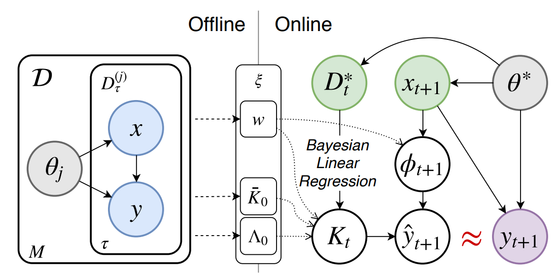
Harrison et al. propose the ALPaCA algorithm that uses an efficient Bayesian linear regression on top of the learned features from the inner optimization loop to represent the mean and variance of that regression as meta-parameters themselves (illustrated in figure 6). The inclusion of prior information here reduces computational complexity and adds more confidence to the final predictions.
哈里森等。提出了一种ALPaCA算法 ，该算法在内部优化循环的学习特征之上使用有效的贝叶斯线性回归，以将回归的均值和方差表示为元参数本身(如图6所示)。此处包含先验信息可降低计算复杂性，并为最终预测增加更多信心。
Bertinetto et al. attempt to solve meta-learning with differentiable closed-form solutions. In particular, they apply a ridge regression as a base learner for the features in the inner optimization loop. The mean and variance predictions from the ridge regression are then used as meta-parameters in the outer optimization loop.
Bertinetto等。尝试用微分封闭式解决方案解决元学习。特别是，他们将岭回归作为内部优化循环中要素的基础学习者。然后，将来自岭回归的均值和方差预测用作外部优化循环中的元参数。

Lee et al. attempt to solve meta-learning with differentiable convex optimization solutions. The proposed method, called MetaOptNet, uses a support vector machine to learn the features from the inner optimization loop (as seen in figure 7).
Lee等。尝试用微分凸优化解决方案解决元学习。提议的方法称为MetaOptNet ，它使用支持向量机从内部优化循环中学习特征(如图7所示)。

4.3 —挑战 (4.3 — Challenges)

The MAML method requires very deep neural architecture in order to effectively get a good inner gradient update. Therefore, the first challenge lies in choosing that architecture. Kim et al. propose Auto-Meta, which searches for the MAML architecture. They found that the highly non-standard architectures with deep and narrow layers tend to perform very well.

MAML方法需要非常深的神经体系结构，以便有效地获得良好的内部梯度更新。因此，第一个挑战在于选择该架构。 Kim等。建议使用Auto-Meta来搜索MAML体系结构。他们发现，具有深层和窄层的高度非标准的体系结构往往表现良好。

The second challenge that comes up lies in the unreliability of the two-degree optimization paradigm. There are many different optimization tricks that can be useful in this scenario:

出现的第二个挑战在于两级优化范式的不可靠性 。在这种情况下，有许多不同的优化技巧可能会有用：

Li et al. propose Meta-SGD that learns the initialization parameters, the direction of the gradient updates, and the value of the inner learning rate in an end-to-end fashion. This method has proven to increase speed and accuracy of the meta-learner.
Li等。提出了以端到端的方式学习初始化参数，梯度更新方向以及内部学习率值的Meta-SGD 。实践证明，这种方法可以提高元学习器的速度和准确性。
Behl et al. come up with Alpha-MAML, which is an extension of the vanilla MAML. Alpha-MAML uses an online hyper-parameter adaptation scheme to automatically tune the learning rate, making the training process more robust.
Behl等。提出Alpha-MAML ，它是香草MAML的扩展。 Alpha-MAML使用在线超参数自适应方案来自动调整学习速率，从而使训练过程更加强大。

Zhou et al. devise Deep Meta-Learning, which performs meta-learning in a concept space. As illustrated in figure 8, the concept generator generates the concept-level features from the inputs, while the concept discriminator distinguishes the features generated from that first step. The final loss function includes both the loss from the discriminator and the loss from the meta-learner.
周等。设计Deep Meta-Learning ，在概念空间中执行元学习。如图8所示，概念生成器从输入生成概念级别的特征，而概念鉴别器则区分从第一步生成的特征。最终损失函数既包括鉴别器的损失，也包括元学习器的损失。
Zintgraf et al. design CAVIA, which stands for fast context adaptation via meta-learning. To handle the overfitting challenge with vanilla MAML, CAVIA optimizes only a subset of the input parameters in the inner loop at test time (deemed context parameters), instead of the whole neural network. By separating the task-specific parameters and task-independent parameters, they show that training CAVIA is highly efficient.
Zintgraf等。 design CAVIA ，它表示通过元学习进行快速上下文适应。为了应对香草MAML的过拟合挑战，CAVIA只会在测试时优化内部循环中输入参数的一个子集(视为上下文参数 )，而不是整个神经网络。通过分离特定于任务的参数和独立于任务的参数，它们表明训练CAVIA是高效的。
Antoniou et al. ideate MAML++, which is a comprehensive guideline on reducing the hyper-parameter sensitivity, lowering the generalization error, and improving MAML stability. One interesting idea is that they disentangle both the learning rate and the batch-norm statistics per step of the inner loop.
Antoniou等。 ideate MAML ++ ，这是降低超参数敏感性，降低泛化误差和提高MAML稳定性的综合指南。一个有趣的想法是，它们使内部循环的每个步骤都无法了解学习率和批次规范统计信息。

In conclusion, optimization-based meta-learning works by constructing a two-degree optimization procedure, where the inner optimization computes the task-specific parameters ϕ and the outer optimization computes the meta-parameters θ. The most representative method is the Model-Agnostic Meta-Learning algorithm, which has been studied and improved upon extensively since its conception.

总之，基于优化的元学习通过构建两级优化程序来进行，其中内部优化计算任务特定参数task，外部优化计算元参数θ。最有代表性的方法是与模型无关的元学习算法，自从概念开始就对其进行了广泛的研究和改进。

The big benefit of MAML is that we can optimize the model’s initialization scheme, in contrast to the black box approach where the initial optimization procedure is not optimized. Furthermore, MAML is highly consistent, which extrapolates well to learning problems where the data is out-of-distribution (compared to what the model has seen during meta-training). Unfortunately, because optimization-based meta-learning requires second-order optimization, it is very computationally expensive.

MAML的最大好处是，我们可以优化模型的初始化方案，这与不优化初始优化程序的黑盒方法相反。此外，MAML具有高度一致性，可以很好地推断出数据分布不当的学习问题(与元训练中模型看到的情况相比)。不幸的是，由于基于优化的元学习需要二阶优化，因此它在计算上非常昂贵。

5 —非参数元学习 (5 — Non-Parametric Meta-Learning)

So can we perform the learning procedure described above without a second-order optimization? This is where non-parametric methods fit in.

那么，我们可以在不进行二阶优化的情况下执行上述学习过程吗？这是适合非参数方法的地方。

Non-parametric methods are very effective at learning with a small amount of data (k-Nearest Neighbor, decision trees, support vector machines). In non-parametric meta-learning, we compare the test data with the training data using some sort of similarity metric. If we find the training data that are most similar to the test data, we assign the labels of those training data as the label of the test data.

非参数方法在学习少量数据(k最近邻，决策树，支持向量机)时非常有效。在非参数元学习中 ，我们使用某种相似性度量将测试数据与训练数据进行比较。如果我们找到与测试数据最相似的训练数据，则将这些训练数据的标签分配为测试数据的标签。

5.1 —配方 (5.1 — Formulation)

This is the non-parametric meta-learning algorithm in a nutshell:

简而言之，这是非参数元学习算法：

We sample a task Tᵢ, as well as the training set Dᵢᵗʳ and test set Dᵢᵗˢ from the task dataset Dᵢ.
我们从任务数据集Dᵢ中采样任务Tᵢ，以及训练集Dᵢᵗʳ和测试集Dᵢᵗˢ。
We predict the test label yᵗˢ via the similarity between training data and test data (represented by f_θ: yᵗˢ = ∑{x_k, y_k ∈ Dᵗʳ} f_θ (xᵗˢ, x_k) y_k.
我们通过训练数据和测试数据之间的相似性来预测测试标签yᵗˢ(用f_θ表示：yᵗˢ= ∑ {x_k， y_k∈Dᵗʳ}f_θ(xᵗˢ，x_k)y_k。
Then we update the meta-parameters θ of this learned embedding function with respect to the loss function of how accurate our predictions are on the test set: ∇_{θ} L(yᵗˢ, yᵗˢ).
然后，相对于我们的预测在测试集上的准确度的损失函数：update_ {θ} L(yᵗˢ，yᵗˢ)，我们更新该学习的嵌入函数的元参数θ。
This process is repeated iteratively with gradient descent optimizers.
使用梯度下降优化器反复重复此过程。

Unlike the black-box and optimization-based approaches, we no longer have the task-specific parameters ϕ, which is not required for the comparison between training and test data.

与基于黑盒和基于优化的方法不同，我们不再具有特定于任务的参数ϕ，这对于训练数据和测试数据之间的比较不是必需的。

5.2 —体系结构 (5.2 — Architectures)

Now let’s go over the different architectures used in non-parametric meta-learning methods.

现在让我们看一下非参数元学习方法中使用的不同体系结构。

Koch et al. propose a Siamese network that consists of two tasks: the verification task and the one-shot task. Taking in pairs of images during training time, the network verifies whether they are of the same class or different classes. At test time, the network performs one-shot learning: comparing each image xᵗˢ to the images in the training set Dⱼᵗʳ for a respective task and predicting the label of xᵗˢ that corresponds to the label of the closest image. Figure 9 illustrates this strategy.

Koch等。提出一个由两个任务组成的暹罗网络 ：验证任务和一次性任务。在训练期间对图像进行成对拍摄，网络将验证它们是相同类别还是不同类别。在测试时，网络执行一次学习：将每个图像xᵗˢ与训练集Dⱼᵗʳ中针对相应任务的图像进行比较，并预测与最接近图像的标签相对应的xᵗˢ标签。图9说明了此策略。

Vinyals et al. propose Matching Networks, which matches the actions happening during training time at test time. The network takes the training data and the test data and embeds them into their respective embedding spaces. Then, the network compares each pair of train-test embeddings to make the final label predictions:

Vinyals等。提出Matching Networks ( 匹配网络) ，以匹配测试时间在训练期间发生的动作。网络获取训练数据和测试数据，并将它们嵌入到各自的嵌入空间中。然后，网络会比较每对训练测试嵌入，以做出最终的标签预测：

The Matching Network architecture used in Matching Networks includes a convolutional encoder network to embed the images and a bi-directional Long-Short Term Memory network to produce the embeddings of such images. As seen in figure 10, the examples in the training set match the examples in the test set.

匹配网络中使用的匹配网络体系结构包括用于嵌入图像的卷积编码器网络和用于生成此类图像的嵌入的双向长短时记忆网络。如图10所示，训练集中的示例与测试集中的示例匹配。

Snell et al. propose Prototypical Networks, which create prototypical embeddings for all the classes in the given data. Then, the network compares those embeddings to make the final label predictions for the corresponding class.

Snell等。提出原型网络 ，该网络为给定数据中的所有类创建原型嵌入。然后，网络将这些嵌入进行比较，以对相应类别进行最终标签预测。

Figure 11 provides a concrete illustration of how Prototypical Networks look like in the few-shot scenario. c₁, c₂, and c₃ are the class prototypical embeddings, which are computed as:

图11提供了在少数情况下原型网络的外观的具体说明。 c₁，c2和c₃是类原型嵌入，其计算公式如下：

Then, we compute the distances from x to each of the prototypical class embeddings: D(fθ(x), c_k).

然后，我们计算从x到每个原型类嵌入的距离： D(fθ(x)，c_ k) 。

To get the final class prediction p_θ(y=k|x), we look at the probability of the negative distances after a softmax activation function, as seen below:

为了获得最终类别预测p_θ(y = k | x)，我们看一下softmax激活函数后负距离的概率，如下所示：

5.3 —挑战 (5.3 — Challenge)

For non-parametric meta-learning, how can we learn deeper interactions between our inputs? The nearest neighbor probably will not work well when our data is high-dimensional. Here are three papers that attempt to accomplish this:

对于非参数元学习， 我们如何学习输入之间的更深层次的互动？ 当我们的数据是高维数据时，最近的邻居可能无法正常工作。这是三篇试图达到这一目的的论文：

Sung et al. come up with RelationNet (figure 12), which has two modules: the embedding module and the relation module. The embedding module embeds the training and test inputs to training and test embeddings. Then the relation module takes in the embeddings and learns a deep distance metric to compare those embeddings (function D in equation 25).
Sung等。提出了RelationNet (图12)，它具有两个模块：嵌入模块和关系模块。嵌入模块将训练和测试输入嵌入到训练和测试嵌入中。然后，关系模块接受嵌入并学习深度距离度量以比较这些嵌入(公式25中的函数D)。
Allen et al. propose an Infinite Mixture of Prototypes. This is an extension of the Prototypical Networks, in the sense that it adaptively sets the model capacity based on the data complexity. By assigning each class its own cluster, this method allows the use of unsupervised clustering, which is helpful for many purposes.
艾伦等。提出原型的无限混合 。这是原型网络的扩展，因为它可以根据数据复杂性自适应地设置模型容量。通过为每个类分配自己的群集，此方法允许使用无监督群集，这对于许多目的都是有帮助的。
Garcia and Bruna use a Graph Neural Network in their meta-learning paradigm. By mapping the inputs into their graphical representation, they can easily learn the similarity between training and test data via the edge and node features.
Garcia和Bruna在他们的元学习范式中使用了Graph Neural Network 。通过将输入映射到其图形表示中，他们可以轻松地通过边缘和节点特征来学习训练数据与测试数据之间的相似性。

六，结论 (6 — Conclusion)

In this post, I have discussed the motivation for meta-learning, the basic formulation and optimization objective for meta-learning, as well as the three approaches regarding the design of the meta-learning algorithm. In particular:

在本文中，我讨论了元学习的动机，元学习的基本公式和优化目标，以及有关元学习算法设计的三种方法。特别是：

Black-box meta-learning algorithms have very strong learning capacity, in the sense that neural networks are universal function approximators. But if we impose certain structures into the function, there is no guarantee that black-box models will produce consistent results. Additionally, we can use black-box approaches with different types of problem settings such as reinforcement learning and self-supervised learning. However, because black-box models always learn from scratch, they are very data-hungry.
在神经网络是通用函数逼近器的意义上， 黑盒元学习算法具有非常强的学习能力。但是，如果我们将某些结构强加给函数，则不能保证黑盒模型会产生一致的结果。此外，我们可以将黑盒方法用于不同类型的问题设置，例如强化学习和自我监督学习。但是，由于黑匣子模型总是从头开始学习，因此它们非常耗费数据。
Optimization-based meta-learning algorithms can be reduced down to gradient descent; thus, it’s reasonable to expect consistent predictions. For deep enough neural networks, optimization-based models also have very high capacity. Because the initialization is optimized internally, optimization-based models have a better head-start than black-box models. Furthermore, we can try out different architectures without any real difficulty, as evidenced by the Model-Agnostic Meta-Learning (MAML) learning paradigm. However, the second-order optimization procedure makes optimization-based approaches quite computationally expensive.
基于优化的元学习算法可以减少到梯度下降。因此，期望一致的预测是合理的。对于足够深的神经网络，基于优化的模型也具有很高的容量。因为初始化是在内部优化的，所以基于优化的模型比黑盒模型具有更好的起点。此外，正如模型不可知元学习(MAML)学习范例所证明的那样，我们可以毫无困难地尝试不同的体系结构。但是，二阶优化过程使基于优化的方法在计算上非常昂贵。
Non-parametric meta-learning algorithms have good learning capacity for most choices of architectures as well as good learning consistency under the assumption that the learned embedding space is effective enough. Furthermore, non-parametric approaches do not involve any back-propagation, so they are computationally fast and easy to optimize. The downside is that they are hard to scale to large batches of data because they are non-parametric.
在学习的嵌入空间足够有效的假设下， 非参数元学习算法对于大多数体系结构选择都具有良好的学习能力，并且具有良好的学习一致性。此外，非参数方法不涉及任何反向传播，因此它们计算快速且易于优化。缺点是它们很难扩展到大批量数据，因为它们是非参数的。

There are a lot of exciting directions for the field of meta-learning, such as Bayesian Meta-Learning (the probabilistic view of meta-learning) and Meta Reinforcement Learning (the use of meta-learning in the reinforcement learning setting). I’d certainly expect to see more real-world applications in wide-ranging domains such as healthcare and manufacturing using meta-learning under the hood. I’d highly recommend going through the course lectures and take detailed notes on the research on these topics!

元学习领域有很多令人振奋的方向，例如贝叶斯元学习(元学习的概率视图)和元强化学习(在强化学习环境中使用元学习)。我当然希望看到在幕后使用元学习的广泛领域，例如医疗保健和制造业中的更多实际应用。我强烈建议您阅读课程讲座，并就这些主题的研究做详细的记录！

该帖子最初发布在我的网站上！ (This post is originally published on my website!)

If you would like to follow my work on Recommendation Systems, Deep Learning, MLOps, and Data Journalism, you can follow my Medium and GitHub, as well as other projects at https://jameskle.com/. You can also tweet at me on Twitter, email me directly, or find me on LinkedIn. Or join my mailing list to receive my latest thoughts right at your inbox!

如果您想关注我在推荐系统，深度学习，MLOps和数据新闻学方面的工作，可以关注我的 Medium 和 GitHub 以及其他项目， 网址为 https://jameskle.com/ 。 您也可以在Twitter在我的 微博， 直接给我发电子邮件 ，或者 找到我的LinkedIn 。或 加入我的邮件目录， 直接在您的收件箱中接收我的最新想法！