


Importing the necessary Libraries and Dataset
## Importing necessary libraries
import pandas as pd
import numpy as np
import matplotlib.pyplot as plt
import seaborn as sns
import datetime
import warnings
warnings.filterwarnings('ignore')
sns.set(style = "whitegrid",font_scale = 1.5)
%matplotlib inline
plt.rcParams['figure.figsize']=[12,8]
#importing Dataset
sensor_df = pd.read_csv('sensor.csv')
Data Wrangling
print("The dataset has " , sensor_df.shape[0],"rows and", sensor_df.shape[1], "columns")
The dataset has  220320 rows and 55 columns
#First 10 rows
sensor_df.head(10)
# Last 10 rows
sensor_df.tail(10)
We have data for sensor readings from April to August, collected daily every minute.
sensor_df.info()
<class 'pandas.core.frame.DataFrame'>
RangeIndex: 220320 entries, 0 to 220319
Data columns (total 55 columns):
 #   Column          Non-Null Count   Dtype
---  ------          --------------   -----
 0   Unnamed: 0      220320 non-null  int64
 1   timestamp       220320 non-null  object
 2   sensor_00       210112 non-null  float64
 3   sensor_01       219951 non-null  float64
 4   sensor_02       220301 non-null  float64
 5   sensor_03       220301 non-null  float64
 6   sensor_04       220301 non-null  float64
 7   sensor_05       220301 non-null  float64
 8   sensor_06       215522 non-null  float64
 9   sensor_07       214869 non-null  float64
 10  sensor_08       215213 non-null  float64
 11  sensor_09       215725 non-null  float64
 12  sensor_10       220301 non-null  float64
 13  sensor_11       220301 non-null  float64
 14  sensor_12       220301 non-null  float64
 15  sensor_13       220301 non-null  float64
 16  sensor_14       220299 non-null  float64
 17  sensor_15       0 non-null       float64
 18  sensor_16       220289 non-null  float64
 19  sensor_17       220274 non-null  float64
 20  sensor_18       220274 non-null  float64
 21  sensor_19       220304 non-null  float64
 22  sensor_20       220304 non-null  float64
 23  sensor_21       220304 non-null  float64
 24  sensor_22       220279 non-null  float64
 25  sensor_23       220304 non-null  float64
 26  sensor_24       220304 non-null  float64
 27  sensor_25       220284 non-null  float64
 28  sensor_26       220300 non-null  float64
 29  sensor_27       220304 non-null  float64
 30  sensor_28       220304 non-null  float64
 31  sensor_29       220248 non-null  float64
 32  sensor_30       220059 non-null  float64
 33  sensor_31       220304 non-null  float64
 34  sensor_32       220252 non-null  float64
 35  sensor_33       220304 non-null  float64
 36  sensor_34       220304 non-null  float64
 37  sensor_35       220304 non-null  float64
 38  sensor_36       220304 non-null  float64
 39  sensor_37       220304 non-null  float64
 40  sensor_38       220293 non-null  float64
 41  sensor_39       220293 non-null  float64
 42  sensor_40       220293 non-null  float64
 43  sensor_41       220293 non-null  float64
 44  sensor_42       220293 non-null  float64
 45  sensor_43       220293 non-null  float64
 46  sensor_44       220293 non-null  float64
 47  sensor_45       220293 non-null  float64
 48  sensor_46       220293 non-null  float64
 49  sensor_47       220293 non-null  float64
 50  sensor_48       220293 non-null  float64
 51  sensor_49       220293 non-null  float64
 52  sensor_50       143303 non-null  float64
 53  sensor_51       204937 non-null  float64
 54  machine_status  220320 non-null  object
dtypes: float64(52), int64(1), object(2)
memory usage: 92.5+ MB
The data set consists of 51 numerical features ,timestamp and a categorical label.


The label contains string values that represent normal, broken and recovering operational conditions of the machine.| count | mean | std | min | 25% | 50% | 75% | max | |
| Unnamed: 0 | 220320.0 | 110159.500000 | 63601.049991 | 0.000000 | 55079.750000 | 110159.500000 | 165239.250000 | 220319.000000 |
| sensor_00 | 210112.0 | 2.372221 | 0.412227 | 0.000000 | 2.438831 | 2.456539 | 2.499826 | 2.549016 |
| sensor_01 | 219951.0 | 47.591611 | 3.296666 | 0.000000 | 46.310760 | 48.133678 | 49.479160 | 56.727430 |
| sensor_02 | 220301.0 | 50.867392 | 3.666820 | 33.159720 | 50.390620 | 51.649300 | 52.777770 | 56.032990 |
| sensor_03 | 220301.0 | 43.752481 | 2.418887 | 31.640620 | 42.838539 | 44.227428 | 45.312500 | 48.220490 |
| sensor_04 | 220301.0 | 590.673936 | 144.023912 | 2.798032 | 626.620400 | 632.638916 | 637.615723 | 800.000000 |
| sensor_05 | 220301.0 | 73.396414 | 17.298247 | 0.000000 | 69.976260 | 75.576790 | 80.912150 | 99.999880 |
| sensor_06 | 215522.0 | 13.501537 | 2.163736 | 0.014468 | 13.346350 | 13.642940 | 14.539930 | 22.251160 |
| sensor_07 | 214869.0 | 15.843152 | 2.201155 | 0.000000 | 15.907120 | 16.167530 | 16.427950 | 23.596640 |
| sensor_08 | 215213.0 | 15.200721 | 2.037390 | 0.028935 | 15.183740 | 15.494790 | 15.697340 | 24.348960 |
| sensor_09 | 215725.0 | 14.799210 | 2.091963 | 0.000000 | 15.053530 | 15.082470 | 15.118630 | 25.000000 |
| sensor_10 | 220301.0 | 41.470339 | 12.093519 | 0.000000 | 40.705260 | 44.291340 | 47.463760 | 76.106860 |
| sensor_11 | 220301.0 | 41.918319 | 13.056425 | 0.000000 | 38.856420 | 45.363140 | 49.656540 | 60.000000 |
| sensor_12 | 220301.0 | 29.136975 | 10.113935 | 0.000000 | 28.686810 | 32.515830 | 34.939730 | 45.000000 |
| sensor_13 | 220301.0 | 7.078858 | 6.901755 | 0.000000 | 1.538516 | 2.929809 | 12.859520 | 31.187550 |
| sensor_14 | 220299.0 | 376.860041 | 113.206382 | 32.409550 | 418.103250 | 420.106200 | 420.997100 | 500.000000 |
| sensor_15 | 0.0 | NaN | NaN | NaN | NaN | NaN | NaN | NaN |
| sensor_16 | 220289.0 | 416.472892 | 126.072642 | 0.000000 | 459.453400 | 462.856100 | 464.302700 | 739.741500 |
| sensor_17 | 220274.0 | 421.127517 | 129.156175 | 0.000000 | 454.138825 | 462.020250 | 466.857075 | 599.999939 |
| sensor_18 | 220274.0 | 2.303785 | 0.765883 | 0.000000 | 2.447542 | 2.533704 | 2.587682 | 4.873250 |
| sensor_19 | 220304.0 | 590.829775 | 199.345820 | 0.000000 | 662.768975 | 665.672400 | 667.146700 | 878.917900 |
| sensor_20 | 220304.0 | 360.805165 | 101.974118 | 0.000000 | 398.021500 | 399.367000 | 400.088400 | 448.907900 |
| sensor_21 | 220304.0 | 796.225942 | 226.679317 | 95.527660 | 875.464400 | 879.697600 | 882.129900 | 1107.526000 |
| sensor_22 | 220279.0 | 459.792815 | 154.528337 | 0.000000 | 478.962600 | 531.855900 | 534.254850 | 594.061100 |
| sensor_23 | 220304.0 | 922.609264 | 291.835280 | 0.000000 | 950.922400 | 981.925000 | 1090.808000 | 1227.564000 |
| sensor_24 | 220304.0 | 556.235397 | 182.297979 | 0.000000 | 601.151050 | 625.873500 | 628.607725 | 1000.000000 |
| sensor_25 | 220284.0 | 649.144799 | 220.865166 | 0.000000 | 693.957800 | 740.203500 | 750.357125 | 839.575000 |
| sensor_26 | 220300.0 | 786.411781 | 246.663608 | 43.154790 | 790.489575 | 861.869600 | 919.104775 | 1214.420000 |
| sensor_27 | 220304.0 | 501.506589 | 169.823173 | 0.000000 | 448.297950 | 494.468450 | 536.274550 | 2000.000000 |
| sensor_28 | 220304.0 | 851.690339 | 313.074032 | 4.319347 | 782.682625 | 967.279850 | 1043.976500 | 1841.146000 |
| sensor_29 | 220248.0 | 576.195305 | 225.764091 | 0.636574 | 518.947225 | 564.872500 | 744.021475 | 1466.281000 |
| sensor_30 | 220059.0 | 614.596442 | 195.726872 | 0.000000 | 627.777800 | 668.981400 | 697.222200 | 1600.000000 |
| sensor_31 | 220304.0 | 863.323100 | 283.544760 | 23.958330 | 839.062400 | 917.708300 | 981.249900 | 1800.000000 |
| sensor_32 | 220252.0 | 804.283915 | 260.602361 | 0.240716 | 760.607475 | 878.850750 | 943.877625 | 1839.211000 |
| sensor_33 | 220304.0 | 486.405980 | 150.751836 | 6.460602 | 489.761075 | 512.271750 | 555.163225 | 1578.600000 |
| sensor_34 | 220304.0 | 234.971776 | 88.376065 | 54.882370 | 172.486300 | 226.356050 | 316.844950 | 425.549800 |
| sensor_35 | 220304.0 | 427.129817 | 141.772519 | 0.000000 | 353.176625 | 473.349350 | 528.891025 | 694.479126 |
| sensor_36 | 220304.0 | 593.033876 | 289.385511 | 2.260970 | 288.547575 | 709.668050 | 837.333025 | 984.060700 |
| sensor_37 | 220304.0 | 60.787360 | 37.604883 | 0.000000 | 28.799220 | 64.295485 | 90.821928 | 174.901200 |
| sensor_38 | 220293.0 | 49.655946 | 10.540397 | 24.479166 | 45.572910 | 49.479160 | 53.645830 | 417.708300 |
| sensor_39 | 220293.0 | 36.610444 | 15.613723 | 19.270830 | 32.552080 | 35.416660 | 39.062500 | 547.916600 |
| sensor_40 | 220293.0 | 68.844530 | 21.371139 | 23.437500 | 57.812500 | 66.406250 | 77.864580 | 512.760400 |
| sensor_41 | 220293.0 | 35.365126 | 7.898665 | 20.833330 | 32.552080 | 34.895832 | 37.760410 | 420.312500 |
| sensor_42 | 220293.0 | 35.453455 | 10.259521 | 22.135416 | 32.812500 | 35.156250 | 36.979164 | 374.218800 |
| sensor_43 | 220293.0 | 43.879591 | 11.044404 | 24.479166 | 39.583330 | 42.968750 | 46.614580 | 408.593700 |
| sensor_44 | 220293.0 | 42.656877 | 11.576355 | 25.752316 | 36.747684 | 40.509260 | 45.138890 | 1000.000000 |
| sensor_45 | 220293.0 | 43.094984 | 12.837520 | 26.331018 | 36.747684 | 40.219910 | 44.849540 | 320.312500 |
| sensor_46 | 220293.0 | 48.018585 | 15.641284 | 26.331018 | 40.509258 | 44.849540 | 51.215280 | 370.370400 |
| sensor_47 | 220293.0 | 44.340903 | 10.442437 | 27.199070 | 39.062500 | 42.534720 | 46.585650 | 303.530100 |
| sensor_48 | 220293.0 | 150.889044 | 82.244957 | 26.331018 | 83.912030 | 138.020800 | 208.333300 | 561.632000 |
| sensor_49 | 220293.0 | 57.119968 | 19.143598 | 26.620370 | 47.743060 | 52.662040 | 60.763890 | 464.409700 |
| sensor_50 | 143303.0 | 183.049260 | 65.258650 | 27.488426 | 167.534700 | 193.865700 | 219.907400 | 1000.000000 |
| sensor_51 | 204937.0 | 202.699667 | 109.588607 | 27.777779 | 179.108800 | 197.338000 | 216.724500 | 1000.000000 |
print('all class labels:',sensor_df['machine_status'].unique())
all class labels: ['NORMAL' 'BROKEN' 'RECOVERING']
The label data has 3 machine status values:
BROKEN represents machine is failed.
RECOVERING represents machine trying to recover from failed status.
NORMAL represents the machine is working in normal status.
#Machine status distribution


sensor_df['machine_status'].value_counts()
NORMAL        205836
RECOVERING     14477
BROKEN             7
Name: machine_status, dtype: int64
Data Preprocessing
Remove redundant columns
Remove duplicates
Handle missing values
Convert Timestamp column which is of type object to datetime
#no values for sensor 15 and unnamed column is unnecessary,so I will drop these columns
sensor_df.drop(['sensor_15','Unnamed: 0'],inplace = True,axis=1)
sensor_df.head()
#check percentage of missing values for each column
(sensor_df.isnull().sum().sort_values(ascending=False)/len(sensor_df))*100
sensor_50         34.956881
sensor_51          6.982117
sensor_00          4.633261
sensor_07          2.474129
sensor_08          2.317992
sensor_06          2.177741
sensor_09          2.085603
sensor_01          0.167484
sensor_30          0.118464
sensor_29          0.032680
sensor_32          0.030864
sensor_17          0.020879
sensor_18          0.020879
sensor_22          0.018609
sensor_25          0.016340
sensor_16          0.014070
sensor_49          0.012255
sensor_48          0.012255
sensor_47          0.012255
sensor_46          0.012255
sensor_45          0.012255
sensor_44          0.012255
sensor_43          0.012255
sensor_42          0.012255
sensor_41          0.012255
sensor_40          0.012255
sensor_39          0.012255
sensor_38          0.012255
sensor_14          0.009532
sensor_26          0.009078
sensor_03          0.008624
sensor_10          0.008624
sensor_13          0.008624
sensor_12          0.008624
sensor_11          0.008624
sensor_05          0.008624
sensor_04          0.008624
sensor_02          0.008624
sensor_36          0.007262
sensor_37          0.007262
sensor_28          0.007262
sensor_27          0.007262
sensor_31          0.007262
sensor_35          0.007262
sensor_24          0.007262
sensor_23          0.007262
sensor_34          0.007262
sensor_21          0.007262
sensor_20          0.007262
sensor_19          0.007262
sensor_33          0.007262
timestamp          0.000000
machine_status     0.000000
dtype: float64
#too many missing values in sensor 50 , so dropping that
sensor_df.drop('sensor_50',inplace = True,axis=1)
sensor_df.head()
to impute some of the missing values with their mean
#imputing the remaining missing values with mean
sensor_df.fillna(sensor_df.mean(),inplace= True)
sensor_df.isnull().sum()
timestamp         0
sensor_00         0
sensor_01         0
sensor_02         0
sensor_03         0
sensor_04         0
sensor_05         0
sensor_06         0
sensor_07         0
sensor_08         0
sensor_09         0
sensor_10         0
sensor_11         0
sensor_12         0
sensor_13         0
sensor_14         0
sensor_16         0
sensor_17         0
sensor_18         0
sensor_19         0
sensor_20         0
sensor_21         0
sensor_22         0
sensor_23         0
sensor_24         0
sensor_25         0
sensor_26         0
sensor_27         0
sensor_28         0
sensor_29         0
sensor_30         0
sensor_31         0
sensor_32         0
sensor_33         0
sensor_34         0
sensor_35         0
sensor_36         0
sensor_37         0
sensor_38         0
sensor_39         0
sensor_40         0
sensor_41         0
sensor_42         0
sensor_43         0
sensor_44         0
sensor_45         0
sensor_46         0
sensor_47         0
sensor_48         0
sensor_49         0
sensor_51         0
machine_status    0
dtype: int64
#checking of duplicate rows

sensor_df.duplicated().any()
False
No duplicate values, hence we don't need to remove any row.
# Now, lets make it a time series and set it as index
sensor_df['timestamp'] = pd.to_datetime(sensor_df['timestamp'])
sensor_df = sensor_df.set_index('timestamp')
The First 5 rows of the dataset looks as follows.
sensor_df.head()
Exploratory Data Analysis
## Machine status distribution
sensor_df.machine_status.value_counts()
NORMAL        205836
RECOVERING     14477
BROKEN             7
Name: machine_status, dtype: int64
#Plotting Machine Status Distribution
plt.figure(figsize=(5,3))
plt.title('machine_status')
sns.countplot(x='machine_status',data=sensor_df)
#machine status -  pie chart
plt.figure(figsize=(5,3))
stroke_labels = ["Normal","Recovering","Broken"]
sizes = sensor_df.machine_status.value_counts()


plt.pie(x=sizes,labels=stroke_labels)
plt.show()
plt.figure(figsize=(60,40))
sns.heatmap(sensor_df.corr(),annot=True,cmap='coolwarm');
corr = sensor_df.corr()
#The HeatMap shows Correlation between features greater than 0.8
corr80 = corr[abs(corr)> 0.8]
sns.heatmap(corr80,cmap='coolwarm')
#extract the readings from the Broken state of the pump
broken= sensor_df[sensor_df['machine_status']=='BROKEN']


#Extract the name of the numerical columns
sensor_df_2 = sensor_df.drop(['machine_status'],axis=1)
names= sensor_df_2.columns


#plot timeseries for each sensor with Broken state marked with X in red color


for name in names:
    _=plt.figure(figsize=(18,3))
    _=plt.plot(broken[name],linestyle='none',marker='X',color='red',markersize=12)
    _=plt.plot(sensor_df[name],color='blue')
    _=plt.title(name)
    plt.show()


#Converting the machine status column to numeric
MS_class_dict = {"BROKEN": 0, "NORMAL": 1, "RECOVERING": 2}
sensor_df['machine_status'] = sensor_df['machine_status'].map(MS_class_dict)
sensor_df.head()
Stationarity and Autocorrelation
# Resample the entire dataset by daily average
rollmean = sensor_df.resample(rule='D').mean()
rollstd = sensor_df.resample(rule='D').std()
# Plot time series for each sensor with its mean and standard deviation with the BROKEN state marked with X in red color
for name in names:
    _ = plt.figure(figsize=(18,3))
    _ = plt.plot(sensor_df[name], color='blue', label='Original')
    _ = plt.plot(rollmean[name], color='red', label='Rolling Mean')
    _ = plt.plot(rollstd[name], color='black', label='Rolling Std' )
    _ = plt.legend(loc='best')
    _ = plt.title(name)
    plt.show()


Pre-processing and Feature Engineering
1.Scale the data
2.Perform PCA and look at the most important principal components based on inertia
# Standardize/scale the dataset and apply PCA
from sklearn.preprocessing import StandardScaler
from sklearn.decomposition import PCA
from sklearn.pipeline import make_pipeline


# Extract the names of the numerical columns
df2 = sensor_df.drop(['machine_status'], axis=1)
names=df2.columns
x = sensor_df[names]
scaler = StandardScaler()
pca = PCA()
pipeline = make_pipeline(scaler, pca)
pipeline.fit(x)
Pipeline(steps=[('standardscaler', StandardScaler()), ('pca', PCA())])
features = range(pca.n_components_)
_ = plt.figure(figsize=(22, 5))
_ = plt.bar(features, pca.explained_variance_)
_ = plt.xlabel('PCA feature')
_ = plt.ylabel('Variance')
_ = plt.xticks(features)
_ = plt.title("Importance of the Principal Components based on inertia")
plt.show()
# Calculate PCA with 2 components
pca = PCA(n_components=2)
principalComponents = pca.fit_transform(x)
principalDf = pd.DataFrame(data = principalComponents, columns = ['pc1', 'pc2'])
principalDf.head()| pc1 | pc2 | |
| 0 | 69.523134 | 265.704571 |
| 1 | 69.523134 | 265.704571 |
| 2 | 27.841569 | 283.462197 |
| 3 | 24.548981 | 290.213914 |
| 4 | 29.627090 | 294.619639 |
sensor_df['pc1']=pd.Series(principalDf['pc1'].values, index=sensor_df.index)
sensor_df['pc2']=pd.Series(principalDf['pc2'].values, index=sensor_df.index)
sensor_df['pc1'],sensor_df['pc2']
(timestamp
 2018-04-01 00:00:00     69.523134
 2018-04-01 00:01:00     69.523134
 2018-04-01 00:02:00     27.841569
 2018-04-01 00:03:00     24.548981
 2018-04-01 00:04:00     29.627090
                           ...
 2018-08-31 23:55:00   -308.531521
 2018-08-31 23:56:00   -294.603672
 2018-08-31 23:57:00   -300.207654
 2018-08-31 23:58:00   -285.141390
 2018-08-31 23:59:00   -298.182526
 Name: pc1, Length: 220320, dtype: float64,
 timestamp
 2018-04-01 00:00:00    265.704571
 2018-04-01 00:01:00    265.704571
 2018-04-01 00:02:00    283.462197
 2018-04-01 00:03:00    290.213914
 2018-04-01 00:04:00    294.619639
                           ...
 2018-08-31 23:55:00   -274.597310
 2018-08-31 23:56:00   -256.328332
 2018-08-31 23:57:00   -256.932727
 2018-08-31 23:58:00   -263.099471
 2018-08-31 23:59:00   -264.545953
 Name: pc2, Length: 220320, dtype: float64)
Check stationarity with Dickey-Fuller Test
# Compute change in daily mean
pca1 = principalDf['pc1'].pct_change()
# Compute autocorrelation
autocorrelation = pca1.dropna().autocorr()
print('Autocorrelation is: ', autocorrelation)
Autocorrelation is:  -6.773604518564134e-06
# Plot ACF
from statsmodels.graphics.tsaplots import plot_acf
plot_acf(pca1.dropna(), lags=20, alpha=0.05)
# Compute change in daily mean
pca2 = principalDf['pc2'].pct_change()
# Compute autocorrelation
autocorrelation = pca2.autocorr()
print('Autocorrelation is: ', autocorrelation)
Autocorrelation is:  -1.4768185278992946e-06
# Plot ACF
from statsmodels.graphics.tsaplots import plot_acf
plot_acf(pca2.dropna(), lags=20, alpha=0.05)
知乎学术咨询:https://www.zhihu.com/consult/people/792359672131756032?isMe=1担任《Mechanical System and Signal Processing》等审稿专家,擅长领域:信号滤波/降噪,机器学习/深度学习,时间序列预分析/预测,设备故障诊断/缺陷检测/异常检测。
分割线
基于自编码器的时间序列异常检测(Python,ipynb文件)
import pandas as pdimport tensorflow as tffrom keras.layers import Input, Densefrom keras.models import Modelfrom sklearn.metrics import precision_recall_fscore_supportimport matplotlib.pyplot as plt
完整代码:
mbd.pub/o/bread/mbd-Zpmcl5xq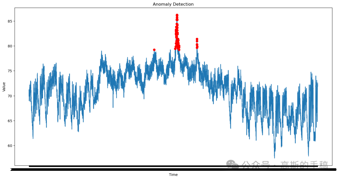


 6459
6459

 被折叠的 条评论
为什么被折叠?
被折叠的 条评论
为什么被折叠?
 到【灌水乐园】发言


