Topic 15. 临床预测模型之决策曲线 (DCA)

最新推荐文章于 2024-04-25 00:03:39 发布

桓峰基因

最新推荐文章于 2024-04-25 00:03:39 发布

阅读量1.4w

点赞数 41

分类专栏： RNA数据分析临床预测模型构建统计学分析方法文章标签：人工智能数据分析数据挖掘

本文链接：https://blog.csdn.net/weixin_41368414/article/details/123723467

版权

RNA数据分析同时被 2 个专栏收录

31 篇文章 61 订阅

订阅专栏

临床预测模型构建统计学分析方法

23 篇文章 123 订阅

订阅专栏

点击关注，桓峰基因

桓峰基因

前言

DCA (Decision Curve Analysis) 是一种评估临床预测模型、诊断试验和分子标记物的简单方法。传统的诊断试验指标如：敏感性，特异性和ROC曲线下面积仅测量预测模型的诊断准确性，未能考虑特定模型的临床效用，而 DCA的优势在于它将患者或决策者的偏好整合到分析中。这种理念的提出满足了临床决策的实际需要，在临床分析中的应用日益广泛。

2006年，MSKCC（纪念斯隆凯特琳癌症研究所）的AndrewVickers博士等人研究出另一种评价方法，叫决策曲线分析法（Decision Curve Analysis，DCA）。相对于二战时期诞生的ROC曲线，DCA还很年轻，也一直在完善之中，不过2012-2020年间，Ann InternMed.、JAMA、BMJ、J Clin Oncol等杂志都已陆续发文，推荐使用决策曲线分析法。

我们在pubmed 中搜索一篇文章，结直肠癌预测临床转移的概率，这篇文章 IF 26分，利用Lasso 回归筛选变量，并且构建模型。

我们看到其中就是分析了模型的DCA决策曲线，可见，模型评估的一些分析在建模类文章中是必不可少的一部分，所以学会了这类文章不用愁，如下：

我们发现临床模型预测之后的评估都需要做决策曲线，基本上临床类分析还是需要做一下，我们看到pubmed上的文章基本上都有，如下：

DCA算法原理

我们先来理解简单的几个概念，只有理解了这些专有词汇，才能够把大数据分析与临床的实际应用结合起来，毕竟发文章只是一种展示科学的一种方式，更高的目标是实施到临床中，挽救更多人的性命，这是一种使命，也是一种责任吧。看定义，如下：

P：给真阳性患者施加干预的受益值（比如用某生化指标预测某患者有癌症，实际也有，予活检，达到了确诊的目的）；

L：给假阳性患者施加干预的损失值（比如预测有癌症，给做了活检，原来只是个增生，白白受了一刀）；

Pi：患者i有癌症的概率，当Pi > Pt时为阳性，给予干预。

所以较为合理的干预的时机是，当且仅当Pi × P >(1 – Pi) × L，即预期的受益高于预期的损失。推导一下可得，Pi > L / ( P + L )即为合理的干预时机，于是把L / ( P + L )定义为Pi的阈值，即Pt。

但对二元的预测指标来说，如果结果是阳性，则强制Pi=1，阴性则Pi = 0。这样，二元和其他类型的指标就有了可比性。

然后我们还可用这些参数来定义真阳性（A）、假阳性（B）、假阴性（C）、真阴性（D），即：

A：Pi ≥ Pt，实际患病；

B：Pi ≥ Pt，实际不患病；

C：Pi < Pt，实际患病；

D：Pi < Pt，实际不患病。

我们有一个随机抽样的样本，A、B、C、D分别为这四类个体在样本中的比例，则A+B+C+D = 1。那么，患病率（π）就是A + C了。

实例解析

我们这里使用三种方法实现决策曲线的绘制，无论方法有几种，最终的结果应该是一致的，这里调用 rmda 和 ggDCA 两个程序包来实现，过程非常详细，仔细运行代码，总会实现的，我发现好多同学都是卡在数据读取，调取，整理数据上，后期也会增加一些此类方法的总结。

1. 软件安装

主要是讲解rmda 和 ggDCA软件包的使用，附加还有rms和caret，程序包安装并加载，这里要注意一下ggDCA安装的时候需要通过git进行安装，否则后面做生存模型时就会不停的报错，如下：

Error in findrow(fit, times, extend) : no points selected for one or more curves, consider using the extend argument

if (!require(rmda)) {
    install.packages("rmda")
}
## Warning: 程辑包'rmda'是用R版本4.1.3 来建造的

if (!require(ggDCA)) {
    devtools::install_github("yikeshu0611/ggDCA")
}
if (!require(rms)) {
    install.packages("rms")
}
if (!require(caret)) {
    install.packages("caret")
}
library(rmda)
library(ggDCA)
library(ggplot2)
library(rms)
library(caret)

2. DCA 曲线绘制

1. plot_decision_curve {rmda}

a.数据读取

我们仍然采用软件包自带的肺癌数据库 NCCTG Lung Cancer Data 作为输入数据，如下：

data(dcaData)
head(dcaData)
## # A tibble: 6 x 6
##     Age Female Smokes Marker1  Marker2 Cancer
##   <int>  <dbl> <lgl>    <dbl>    <dbl>  <int>
## 1    33      1 FALSE    0.245  1.02         0
## 2    29      1 FALSE    0.943 -0.256        0
## 3    28      1 FALSE    0.774  0.332        0
## 4    27      0 FALSE    0.406 -0.00569      0
## 5    23      1 FALSE    0.508  0.208        0
## 6    35      1 FALSE    0.186  1.41         0

b. 模型构建

rmda 软件包自带模型构建函数decision_curve ，构建Logistic 回归模型，

Description

This function calculates decision curves, which are estimates of the standardized net benefit by the probability threshold used to categorize observations as ‘high risk.’ Curves can be estimated using data from an observational cohort (default), or from case-control studies when an estimate of the population outcome prevalence is available. Confidence intervals calculated using the bootstrap are calculated as well.

我们再看下整个函数合适分析哪种模型，很明显，因变量为二分类的数据，1为case，0为controls的数据才可以使用，自变量属性可以是多样性的。

formula | an object of class ‘formula’ of the form outcome ~ predictors, giving the prediction model to be fitted using glm. The outcome must be a binary variable thatequals ‘1’ for cases and ‘0’ for controls.

我们根据数据情况，构建一个基本的二分类模型，如下：

set.seed(123)
baseline.model <- decision_curve(Cancer ~ Age + Female + Smokes, data = dcaData,
    thresholds = seq(0, 0.4, by = 0.005), bootstraps = 10)

c.DCA曲线绘制

单个模型绘制DCA决策曲线，如下：

plot_decision_curve(baseline.model,  
                    curve.names = "Baseline Model",
                    cost.benefit.axis =FALSE,
                    #col= c('red','blue'),
                    confidence.intervals=FALSE,
                    standardize = FALSE)

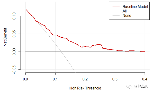
Figure 1: Decision Curve Analysis of Baseline Model

在构造一个全变量模型，及将其他剩余的变量都加入模型中，构建预测模型并做图，如下：

set.seed(123)
full.model <- decision_curve(Cancer~Age + Female + Smokes + Marker1 + Marker2,
                             data = dcaData,
                             thresholds = seq(0, .4, by = .005),
                             bootstraps = 10)
plot_decision_curve(full.model,  
                    curve.names = "Full Model",
                    cost.benefit.axis =FALSE,
                    #col= c('red','blue'),
                    confidence.intervals=FALSE,
                    standardize = FALSE)

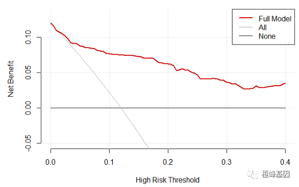
Figure 2: Decision Curve Analysis of Full Model

d.多模型同图

那么我们需要将两个构建好的模型放在一张图上，以此来比较两个模型的性能，如下：

plot_decision_curve(list(baseline.model, full.model), curve.names = c("Baseline model",
    "Full model"), col = c("blue", "red"), lty = c(1, 2), lwd = c(3, 2, 2, 1), legend.position = "bottomright")

‍

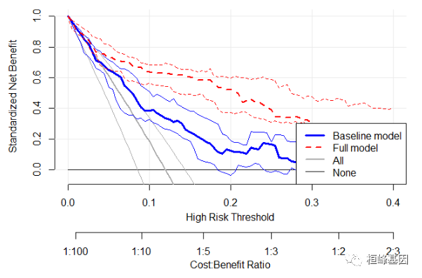
‍p‍‍

Figure 3: Decision Curve Analysis of two Models

我们不需要那么复杂，只需要显示两个模型的预测曲线即可，如下：

plot_decision_curve( list(baseline.model, full.model),
                    curve.names = c("Baseline model", "Full model"),
                    col = c("blue", "red"),
                    confidence.intervals = FALSE,  #remove confidence intervals
                    cost.benefit.axis = FALSE, #remove cost benefit axis
                    legend.position = "topright") #add the legend

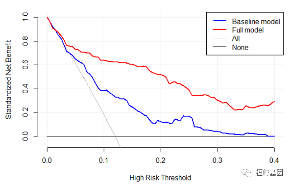
Figure 4: Decision Curve Analysis of Two Models

2. dca {ggDCA}

a.数据读取

我们调取ggDCA程序包里面数据，为肝癌数据，并且里面含有四个关键基因(ANLN，CENPA，GPR182，BCO2及生存信息(结局变量(status)，生存时间(time))，共232个患者，我们利用这套数据构建 Cox 回归模型，并绘制DCA决策曲线。

ICGC Liver Data from Japan

Description

This data is a liver cancer data from Japan Data released in ICGC database (Link). It cantains time, event and four genes.

Format

An object of class data.frame with 232 rows and 6 columns.

将数据切分成测试集和验证集，以方便我们做验证，如下：

data(LIRI)
head(LIRI)
##        time status      ANLN     CENPA     GPR182      BCO2
## 1 3.0410959      1  6.821354 3.0366550 0.00000000 0.2248344
## 2 2.5479452      0  1.073527 0.4654169 0.17895040 5.8924860
## 3 4.0273973      0  2.579530 0.7732644 0.06809686 3.5994330
## 4 0.1643836      1 14.183630 7.7239000 0.03749626 1.1194870
## 5 0.8219178      0  3.588320 2.3237710 0.16762610 2.6660850
## 6 2.8767123      0  6.079665 3.6674980 0.21788230 0.7691067
ddist <- datadist(LIRI)  ###打包数据
options(datadist = "ddist")

b.模型构建

程序包ggDCA 中dca可以单个或多个模型的DCA曲线绘制，模型对象包括四个：

coxph (Cox 比例风险回归模型,Fit Proportional Hazards Regression Model)
cph (Cox 比例风险回归模型,Cox Proportional Hazards Model and Extensions)
glm (广义线型模型,Fitting Generalized Linear Models）
lrm (逻辑回归模型,Logistic Regression Model)

同时还可以设置不同时期的预测效果，也可以在验证集里面进行验证。

one or more results of logistic or cox regression

c.DCA绘制

构建Logistic回归模型

根据不同情况，添加变量即为基因的个数，构建四个不同变量的Logistic 回归模型。

构建4个logstic模型lrm1,lrm2,lrm3,lrm4,模型的变量一次递加基因个数，如下：

lrm1 <- lrm(status ~ ANLN, LIRI)
lrm2 <- lrm(status ~ ANLN + CENPA, LIRI)
lrm3 <- lrm(status ~ ANLN + CENPA + GPR182, LIRI)
lrm4 <- lrm(status ~ ANLN + CENPA + GPR182 + BCO2, LIRI)

我们看一下结果，包括阈值，真阳性，假阳性，净收益，模型名称，如下：

dca_lrm <- dca(lrm1, lrm2, lrm3, lrm4, model.names = c("ANLN", "ANLN+CENPA", "ANLN+CENPA+GPR182",
    "ANLN+CENPA+GPR182+BCO2"))
head(dca_lrm)
##   thresholds       TPR       FPR        NB model
## 1 0.07825978 0.1853448 0.8146552 0.1161770  ANLN
## 2 0.08070249 0.1853448 0.8103448 0.1142070  ANLN
## 3 0.08080998 0.1853448 0.8060345 0.1144828  ANLN
## 4 0.08132494 0.1810345 0.8060345 0.1096810  ANLN
## 5 0.08191934 0.1810345 0.8017241 0.1094975  ANLN
## 6 0.08240994 0.1810345 0.7974138 0.1094177  ANLN

绘制DCA曲线，如下：

ggplot(dca_lrm, lwd = 0.5)

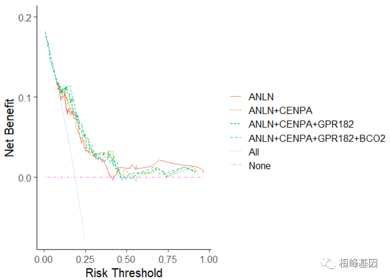
Figure 5: Decision Curve Analysis of Multi Logistic Models

构建Cox回归模型

根据不同情况，添加变量即为基因的个数，构建四个不同变量的Cox回归模型。

构建4个Cox回归模型cph1,cph2,cph3,cph4,模型的变量一次递加基因个数，如下：

cph1 <- cph(Surv(time, status) ~ ANLN, LIRI)
cph2 <- cph(Surv(time, status) ~ ANLN + CENPA, LIRI)
cph3 <- cph(Surv(time, status) ~ ANLN + CENPA + GPR182, LIRI)
cph4 <- cph(Surv(time, status) ~ ANLN + CENPA + GPR182 + BCO2, LIRI)

我们看一下结果，包括阈值，真阳性，假阳性，净收益，时间，模型名称，如下：

dca_cph <- dca(cph1, cph2, cph3, cph4, model.names = c("ANLN", "ANLN+CENPA", "ANLN+CENPA+GPR182",
    "ANLN+CENPA+GPR182+BCO2"))
head(dca_cph)
##   thresholds       TPR       FPR         NB     time model
## 1 0.08642800 0.1694905 0.8305095 0.09092056 2.136986  ANLN
## 2 0.08837278 0.1696432 0.8260465 0.08956656 2.136986  ANLN
## 3 0.08845805 0.1697980 0.8215813 0.09006990 2.136986  ANLN
## 4 0.08886622 0.1654711 0.8215979 0.08533766 2.136986  ANLN
## 5 0.08933664 0.1656280 0.8171306 0.08546698 2.136986  ANLN
## 6 0.08972435 0.1657871 0.8126612 0.08568445 2.136986  ANLN


ggplot(dca_cph, lwd = 0.5)

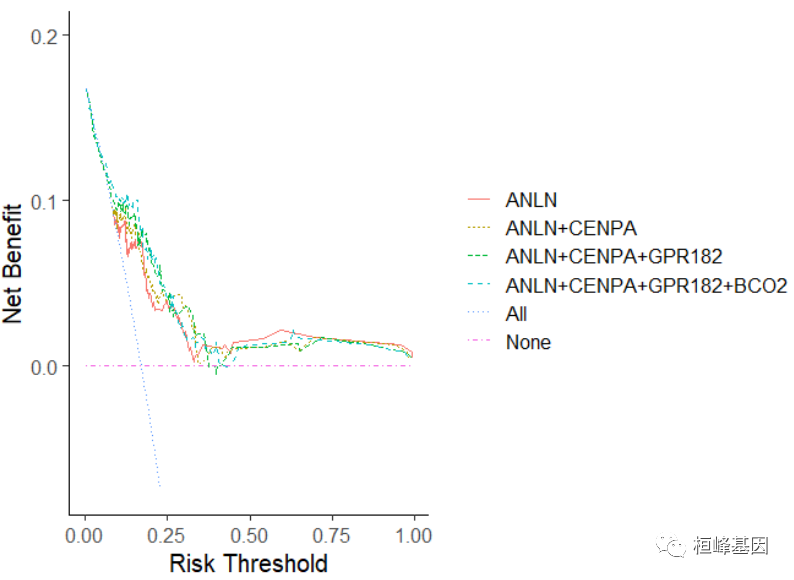
Figure 6: Decision Curve Analysis of Multi Cox Models.

除此之外，还有关于生存Cox回归模型，我们还可以选择几种不同时间点以及在验证集中验证等都非常的方便，下面来自公众号：一棵树，于老师的分享，我这里直接借用一下。

1.单个模型，不给times赋值，默认验证中位时间

dca_cph <- dca(cph1, model.names = "ANLN")
ggplot(dca_cph)

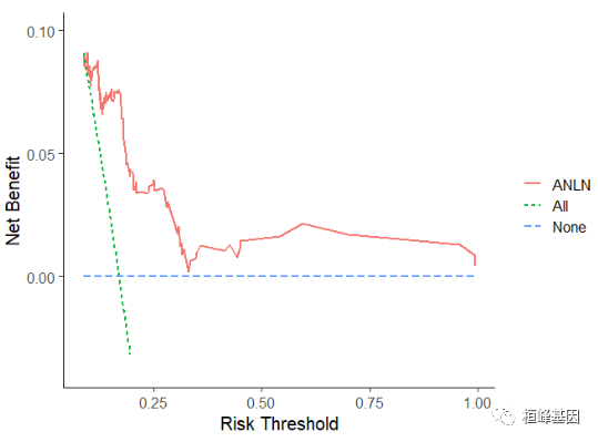
Figure 7: Decision Curve Analysis of Single Model in the time point of median.

2.单个模型，多个时间点(生存时间的下四分位数、中位数、上四分位数)

times = round(quantile(LIRI$time, c(0.25, 0.5, 0.75)), 2)
dca_cph <- dca(cph1, model.names = "ANLN", times = times)
ggplot(dca_cph)

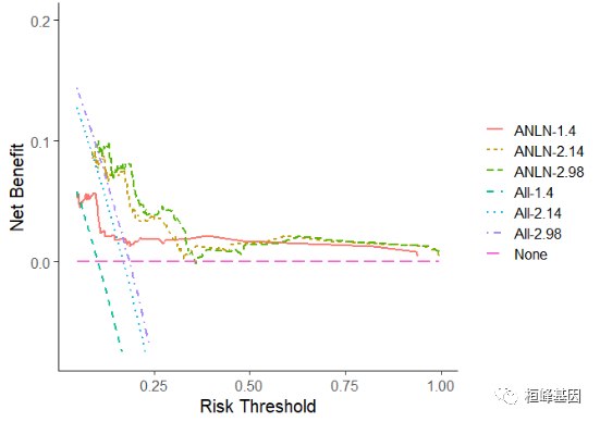
Figure 8: Decision Curve Analysis of Single Cox Models in different time points.

3.多个模型，同一个时间点

dca_cph <- dca(cph1, cph2, cph3, cph4, model.names = c("ANLN", "ANLN+CENPA", "ANLN+CENPA+GPR182",
    "ANLN+CENPA+GPR182+BCO2"), times = 2)
ggplot(dca_cph)

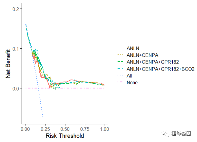
Figure 9: Decision Curve Analysis of Multi Cox Models in the same time point.

4.多个模型，多个时间点

dca_cph <- dca(cph1, cph2, cph3, cph4, model.names = c("ANLN", "ANLN+CENPA", "ANLN+CENPA+GPR182",
    "ANLN+CENPA+GPR182+BCO2"), times = c(1.5, 2, 3))
ggplot(dca_cph)

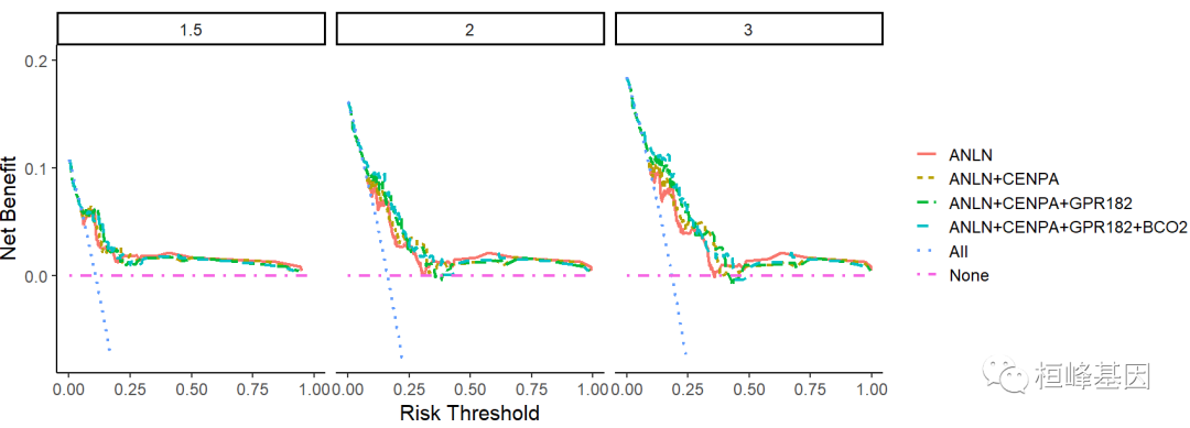
Figure 10: Decision Curve Analysis of Multi Cox Models in different times points

结果解读

DCA曲线图的横坐标为阈概率（ThresholdProbability）。当各种评价方法达到某个值时，患者i的死亡风险概率记为Pi；当Pi达某个阈值（记为Pt），就界定为阳性，采取某种干预措施。纵坐标就是利减去弊之后的净获益率。

另外还有一个包 dcurves同样可以绘制DCA曲线图，但是个人感觉有点复杂，所以就没推荐，感觉这些足以满足需求。不知道大家看懂了没，仔细推敲还是很好理解，关注公众号，桓峰基因，每天更新不停歇！

References:

Vickers AJ, Elkin EB. Decision curve analysis: a novel method for evaluating prediction models. Med Decis Making. 2006;26(6):565-574.
Vickers AJ, van Calster B, Steyerberg EW. A simple, step-by-step guide to interpreting decision curve analysis. Diagn Progn Res. 2019;3:18. Published 2019 Oct 4.
Van Calster B, Wynants L, Verbeek JFM, et al. Reporting and Interpreting Decision Curve Analysis: A Guide for Investigators.Eur Urol. 2018;74(6):796-804.