SCS【22】单细胞转录组之 RNA 速度估计 (Velocyto.R)

最新推荐文章于 2024-04-21 07:24:02 发布

桓峰基因

最新推荐文章于 2024-04-21 07:24:02 发布

阅读量921

点赞数

文章标签： r语言开发语言

本文链接：https://blog.csdn.net/weixin_41368414/article/details/130279185

版权

桓峰基因公众号推出单细胞生信分析教程并配有视频在线教程，目前整理出来的相关教程目录如下：

Topic 6. 克隆进化之 Canopy

Topic 7. 克隆进化之 Cardelino

Topic 8. 克隆进化之 RobustClone

SCS【1】今天开启单细胞之旅，述说单细胞测序的前世今生

SCS【2】单细胞转录组之 cellranger

SCS【3】单细胞转录组数据 GEO 下载及读取

SCS【4】单细胞转录组数据可视化分析 (Seurat 4.0)

SCS【5】单细胞转录组数据可视化分析 (scater)

SCS【6】单细胞转录组之细胞类型自动注释 (SingleR)

SCS【7】单细胞转录组之轨迹分析 (Monocle 3) 聚类、分类和计数细胞

SCS【8】单细胞转录组之筛选标记基因 (Monocle 3)

SCS【9】单细胞转录组之构建细胞轨迹 (Monocle 3)

SCS【10】单细胞转录组之差异表达分析 (Monocle 3)

SCS【11】单细胞ATAC-seq 可视化分析 (Cicero)

SCS【12】单细胞转录组之评估不同单细胞亚群的分化潜能 (Cytotrace)

SCS【13】单细胞转录组之识别细胞对“基因集”的响应 (AUCell)

SCS【14】单细胞调节网络推理和聚类 (SCENIC)

SCS【15】细胞交互：受体-配体及其相互作用的细胞通讯数据库 (CellPhoneDB)

SCS【16】从肿瘤单细胞RNA-Seq数据中推断拷贝数变化 (inferCNV)

SCS【17】从单细胞转录组推断肿瘤的CNV和亚克隆 (copyKAT)

SCS【18】细胞交互：受体-配体及其相互作用的细胞通讯数据库 (iTALK)

SCS【19】单细胞自动注释细胞类型 (Symphony)

SCS【20】单细胞数据估计组织中细胞类型(Music)

SCS【21】单细胞空间转录组可视化 (Seurat V5)

简介

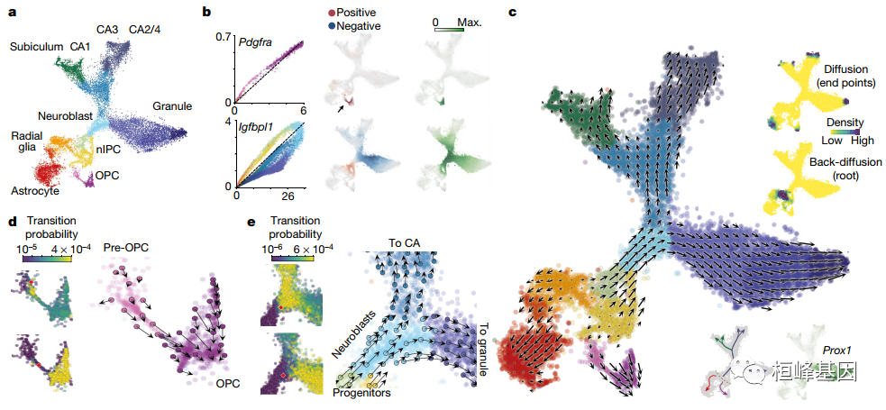
RNA丰度是单个细胞状态的有力指标。单细胞RNA测序可显示RNA丰度，具有较高的定量准确性、灵敏度和通量。然而，这种方法只能捕获某个时间点的静态快照，这对胚胎发生或组织再生等时间分辨现象的分析提出了挑战。在这里，我们展示了RNA速度——基因表达状态的时间导数——可以通过区分普通单细胞RNA测序方案中未剪接和剪接的mRNA来直接估计。RNA速度是一种高维矢量，可以在小时的时间尺度上预测单个细胞的未来状态。我们验证了其在神经嵴谱系中的准确性，展示了其在多个已发表的数据集和技术平台上的使用，揭示了发育中的小鼠海马的分支谱系树，并检查了人类胚胎大脑的转录动力学。我们期望RNA速度能够极大地帮助分析发育谱系和细胞动力学，特别是在人类中。

参考官网说明：

http://pklab.med.harvard.edu/velocyto/notebooks/R/DG1.nb.html

软件包安装

在window上安装velocyto.R软件包相对比较麻烦，需要在安装之前依赖几款软件，安装顺序为：Microsoft Visual Studio ———> Boost ———> velocyto.R。若出现一些问题可以看桓峰基因公众号上的教程：

软件安装系列：Boost 的安装与初试

软件安装系列：R velocyto.R 的安装与初试

library(devtools)
if (!require(velocyto.R)) devtools::install_github("velocyto-team/velocyto.R")

if (!require(pagoda2)) install.packages("pagoda2")
# or
if (!require(pagoda2)) devtools::install_github("kharchenkolab/pagoda2")

数据读取

该示例展示了从velocyto.R准备的矩阵中加载拼接/未拼接的矩阵，使用pagoda2聚类/嵌入细胞，然后可视化该嵌入上的RNA速度。

这个 .loom 文件可以通过 velocyto.py 获取，R 版的搞不定这么大的数据，需要预先使用Python处理之后获得loom文件，具体过程见官方教程：

http://velocyto.org/velocyto.py/tutorial/cli.html#run-smartseq2-run-on-smartseq2-samples

我们直接使用现成的loom文件，数据下载：

http://pklab.med.harvard.edu/velocyto/DG1/10X43_1.loom

文件说明：

The loom file is simply an HDF5 file with a strict structure imposed on it. This structure helps keep consistency in an otherwise unordered binary file and provides security in the knowledge of which data is which. Below is a summary of the file structure and rules imposed on each dataset; for more details, please read the loom file specification.

matrix: The root of a loom file’s structure, it has two dimensions of (n) genes and (m) cells

layers: Alternative representations of the data in matrix, must have the same dimensions as matrix

row_attrs and col_attrs Metadata for rows (genes) and columns (cells), respectively; each dataset in these groups must be one- or two-dimensional and the first dimension must be (n) for row_attrs or (m) forcol_attrs

row_graphs and col_graphs Sparse cluster graphs in coordinate form; each graph is a group with three equal-length datasets: a (row index), b (column index), and w (value)

library(Seurat)
options(Seurat.object.assay.version = "v5")
library(velocyto.R)
ldat <- read.loom.matrices("10X43_1.loom")
## reading loom file via hdf5r...

实例操作

使用pagoda2标准化和聚集细胞

使用拼接表达式矩阵作为pagoda2的输入：

emat <- ldat$spliced
emat <- emat[, colSums(emat) >= 1000]

Pagoda2处理

Pagoda2用于生成细胞嵌入、细胞聚类以及更精确的细胞-细胞距离矩阵。也可以使用其他工具(如Seurat等)生成它们。

创建pagoda2对象，调整方差:

library(pagoda2)
r <- Pagoda2$new(emat, modelType = "plain", trim = 10, log.scale = T)
r$adjustVariance(plot = T, do.par = T, gam.k = 10)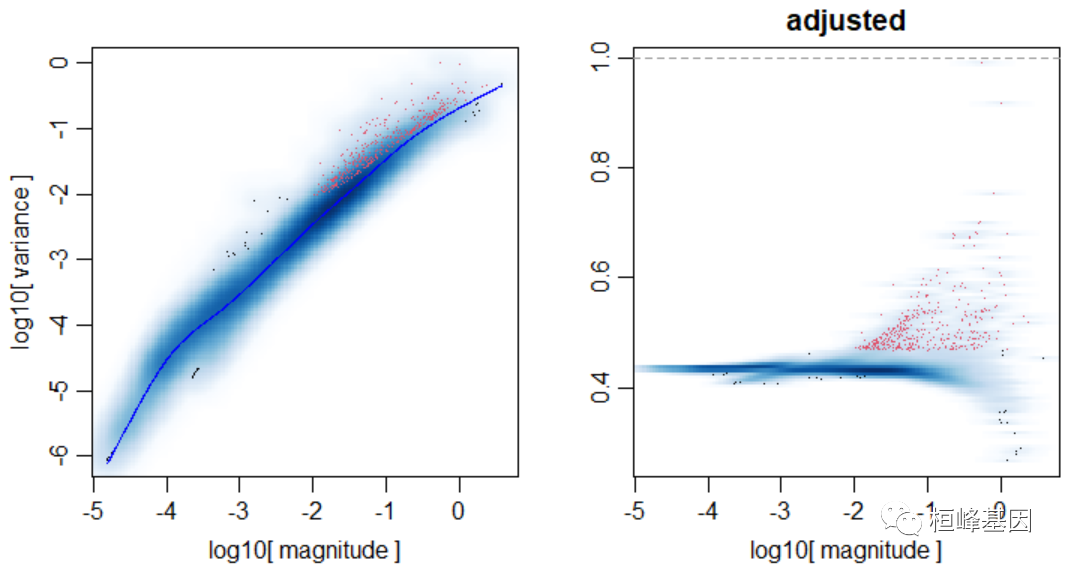

运行基本分析步骤，生成细胞嵌入和聚类，可视化:

r$calculatePcaReduction(nPcs = 100, n.odgenes = 3000, maxit = 300)
r$makeKnnGraph(k = 30, type = "PCA", center = T, distance = "cosine")
## creating space of type angular done
## adding data ... done
## building index ... done
## querying ... done
r$getKnnClusters(method = multilevel.community, type = "PCA", name = "multilevel")
r$getEmbedding(type = "PCA", embeddingType = "tSNE", perplexity = 50, verbose = T)

绘图，标记簇(左)和“Xist”表达(区分男性和女性)

par(mfrow = c(1, 2))
r$plotEmbedding(type = "PCA", embeddingType = "tSNE", show.legend = F, mark.clusters = T,
    min.group.size = 10, shuffle.colors = F, mark.cluster.cex = 1, alpha = 0.3, main = "cell clusters")

r$plotEmbedding(type = "PCA", embeddingType = "tSNE", colors = r$counts[, "Xist"],
    main = "Xist")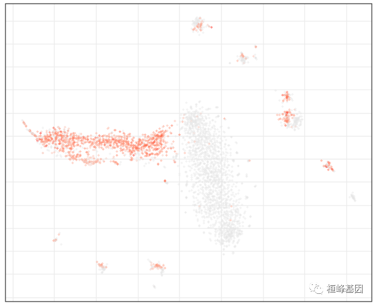

速度估计

准备矩阵和聚类数据:

emat <- ldat$spliced
nmat <- ldat$unspliced
emat <- emat[,rownames(r$counts)]; nmat <- nmat[,rownames(r$counts)]; # restrict to cells that passed p2 filter
# take cluster labels
cluster.label <- r$clusters$PCA[[1]]
cell.colors <- sccore::fac2col(cluster.label)
# take embedding
emb <- r$embeddings$PCA$tSNE

除了聚类和t-SNE嵌入外，我们还将从p2处理中取一个细胞-细胞距离，这将优于velocyto默认的全转录组相关距离。

cell.dist <- as.dist(1 - armaCor(t(r$reductions$PCA)))

根据最小平均表达量(在至少一个簇中)筛选基因，输出得到的有效基因总数:

emat <- filter.genes.by.cluster.expression(emat, cluster.label, min.max.cluster.average = 0.5)
nmat <- filter.genes.by.cluster.expression(nmat, cluster.label, min.max.cluster.average = 0.05)
length(intersect(rownames(emat), rownames(emat)))
## [1] 3712

估计RNA速度(使用k=20细胞kNN池化的基因相关模型，并使用顶部/底部2%分位数进行伽马拟合):

fit.quantile <- 0.02
rvel.cd <- gene.relative.velocity.estimates(emat, nmat, deltaT = 1, kCells = 20,
    cell.dist = cell.dist, fit.quantile = fit.quantile, n.cores = 1)
## calculating cell knn ... done
## calculating convolved matrices ... done
## fitting gamma coefficients ... done. succesfful fit for 1239 genes
## filtered out 171 out of 1239 genes due to low nmat-emat correlation
## filtered out 137 out of 1068 genes due to low nmat-emat slope
## calculating RNA velocity shift ... done
## calculating extrapolated cell state ... done

使用速度矢量可视化t-SNE嵌入上的速度:

show.velocity.on.embedding.cor(emb, rvel.cd, n = 300, scale = "sqrt", cell.colors = ac(cell.colors,
    alpha = 0.5), cex = 0.8, arrow.scale = 5, show.grid.flow = TRUE, min.grid.cell.mass = 0.5,
    grid.n = 40, arrow.lwd = 1, do.par = F, cell.border.alpha = 0.1)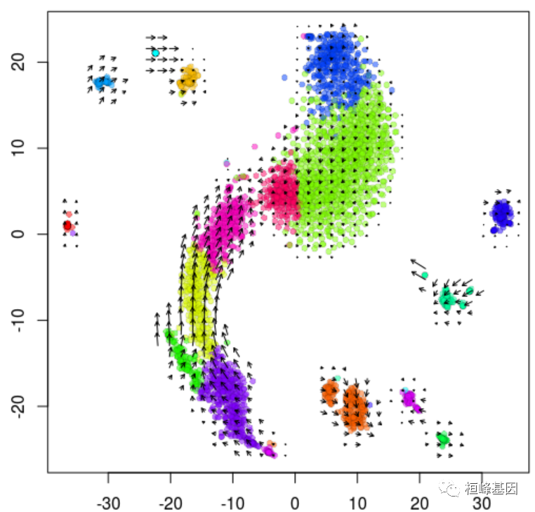

## delta projections ... sqrt knn ... transition probs ... done
## calculating arrows ... done
## grid estimates ... grid.sd= 1.242266  min.arrow.size= 0.02484532  max.grid.arrow.length= 0.04106168  done

假色一个适合特定基因的人(重复使用rvel):

gene <- "Nfib"
gene.relative.velocity.estimates(emat, nmat, deltaT = 1, kCells = 20, kGenes = 1,
    fit.quantile = fit.quantile, cell.emb = emb, cell.colors = cell.colors, cell.dist = cell.dist,
    show.gene = gene, old.fit = rvel.cd, do.par = T)
## calculating convolved matrices ... done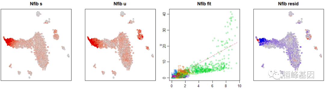

## [1] 1

Reference

La Manno, G., Soldatov, R., Zeisel, A. et al. RNA velocity of single cells. Nature 560, 494–498 (2018). https://doi.org/10.1038/s41586-018-0414-6

这个软件包代码量还是很多的，需要具有一定 R 语言编程基础，并不是看起来那么简单，所有好多老师想直接自己学习教程来分析，但是实质上没有基础还是很难实现，每步报错都不知道该怎样处理，是最崩溃的，所以有需求的老师可以联系桓峰基因，提供最优质的服务！！！

桓峰基因，铸造成功的您！

未来桓峰基因公众号将不间断的推出单细胞系列生信分析教程，

敬请期待！！

桓峰基因和投必得合作，文章润色优惠85折，需要文章润色的老师可以直接到网站输入领取桓峰基因专属优惠券码：KYOHOGENE，然后上传，付款时选择桓峰基因优惠券即可享受85折优惠哦！https://www.topeditsci.com/

有想进生信交流群的老师可以扫最后一个二维码加微信，备注“单位+姓名+目的”!!!

桓峰基因

关注

0
点赞
踩
8

收藏

觉得还不错? 一键收藏
0
评论
SCS【22】单细胞转录组之 RNA 速度估计 (Velocyto.R)

桓峰基因公众号推出单细胞生信分析教程并配有视频在线教程，目前整理出来的相关教程目录如下：Topic 6. 克隆进化之 CanopyTopic 7. 克隆进化之 CardelinoTopic 8. 克隆进化之 RobustCloneSCS【1】今天开启单细胞之旅，述说单细胞测序的前世今生SCS【2】单细胞转录组之 cellrangerSCS【3】单细胞转录组数据 GEO 下载及读取SCS【4】单细...
复制链接

扫一扫