


这期介绍一下NB的最佳集成分类方法之一 AdaBoost,并实现在具体数据集上的应用,尤其是临床数据。
简 介
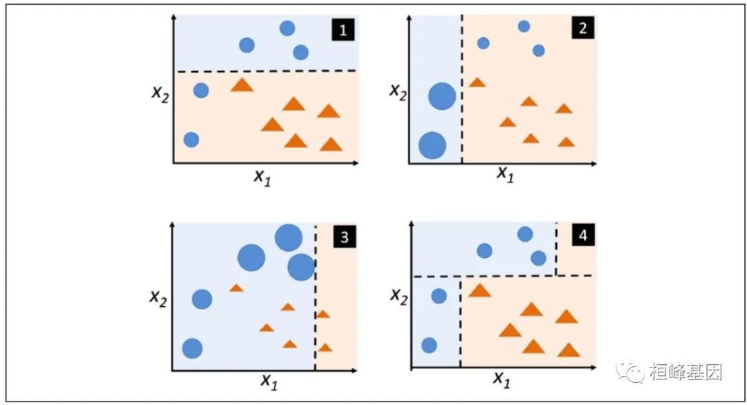
Adaboost是Adaptive Boosting的缩写,使用一组简单的弱分类器,通过强调被弱分类器错误分类的样本来实现改进的分类器。AdaBoost是一种集成模型,使用的是boosting框架思想。
首先,让我们回顾一下原始的增强算法过程:
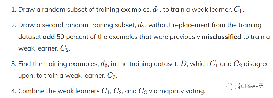
与原始的增强过程相反,AdaBoost使用完整的训练数据集来训练弱学习器,其中训练示例在每次迭代中重新加权,以构建一个强分类器,该分类器从集成中先前弱学习器的错误中学习。

软件安装
这里我们主要介绍caret,另外还有两个包同样可以实现Adaboost算法,软件包安装方法如下:
install.packages('caret')
install.packages('skimr')
install.packages("adabag")
devtools::install_github("souravc83/fastAdaboost")
devtools::install_github('ramnathv/rCharts')
数据读取
这里我们选择之前在分析机器学习曾经使用过的数据集:BreastCancer,可以跟我们之前的方法对比一下:
基于机器学习构建临床预测模型
MachineLearning 2. 因子分析(Factor Analysis)
MachineLearning 3. 聚类分析(Cluster Analysis)
MachineLearning 4. 癌症诊断方法之 K-邻近算法(KNN)
MachineLearning 5. 癌症诊断和分子分型方法之支持向量机(SVM)
MachineLearning 6. 癌症诊断机器学习之分类树(Classification Trees)
MachineLearning 7. 癌症诊断机器学习之回归树(Regression Trees)
MachineLearning 8. 癌症诊断机器学习之随机森林(Random Forest)
MachineLearning 9. 癌症诊断机器学习之梯度提升算法(Gradient Boosting)
MachineLearning 10. 癌症诊断机器学习之神经网络(Neural network)
MachineLearning 11. 机器学习之随机森林生存分析(randomForestSRC)
library(ggplot2)
library(dplyr)
library(tidyverse)
library(pROC)
library(caret)
library(fastAdaboost)
library(caret)
### 分类型
BreastCancer <- read.csv("wisc_bc_data.csv", stringsAsFactors = FALSE)
dim(BreastCancer)
## [1] 568  32
str(BreastCancer)
## 'data.frame':	568 obs. of  32 variables:
##  $ id                     : int  842517 84300903 84348301 84358402 843786 844359 84458202 844981 84501001 845636 ...
##  $ diagnosis              : chr  "M" "M" "M" "M" ...
##  $ radius_mean            : num  20.6 19.7 11.4 20.3 12.4 ...
##  $ texture_mean           : num  17.8 21.2 20.4 14.3 15.7 ...
##  $ perimeter_mean         : num  132.9 130 77.6 135.1 82.6 ...
##  $ area_mean              : num  1326 1203 386 1297 477 ...
##  $ smoothness_mean        : num  0.0847 0.1096 0.1425 0.1003 0.1278 ...
##  $ compactne_mean         : num  0.0786 0.1599 0.2839 0.1328 0.17 ...
##  $ concavity_mean         : num  0.0869 0.1974 0.2414 0.198 0.1578 ...
##  $ concave_points_mean    : num  0.0702 0.1279 0.1052 0.1043 0.0809 ...
##  $ symmetry_mean          : num  0.181 0.207 0.26 0.181 0.209 ...
##  $ fractal_dimension_mean : num  0.0567 0.06 0.0974 0.0588 0.0761 ...
##  $ radius_se              : num  0.543 0.746 0.496 0.757 0.335 ...
##  $ texture_se             : num  0.734 0.787 1.156 0.781 0.89 ...
##  $ perimeter_se           : num  3.4 4.58 3.44 5.44 2.22 ...
##  $ area_se                : num  74.1 94 27.2 94.4 27.2 ...
##  $ smoothness_se          : num  0.00522 0.00615 0.00911 0.01149 0.00751 ...
##  $ compactne_se           : num  0.0131 0.0401 0.0746 0.0246 0.0335 ...
##  $ concavity_se           : num  0.0186 0.0383 0.0566 0.0569 0.0367 ...
##  $ concave_points_se      : num  0.0134 0.0206 0.0187 0.0188 0.0114 ...
##  $ symmetry_se            : num  0.0139 0.0225 0.0596 0.0176 0.0216 ...
##  $ fractal_dimension_se   : num  0.00353 0.00457 0.00921 0.00511 0.00508 ...
##  $ radius_worst           : num  25 23.6 14.9 22.5 15.5 ...
##  $ texture_worst          : num  23.4 25.5 26.5 16.7 23.8 ...
##  $ perimeter_worst        : num  158.8 152.5 98.9 152.2 103.4 ...
##  $ area_worst             : num  1956 1709 568 1575 742 ...
##  $ smoothness_worst       : num  0.124 0.144 0.21 0.137 0.179 ...
##  $ compactne_worst        : num  0.187 0.424 0.866 0.205 0.525 ...
##  $ concavity_worst        : num  0.242 0.45 0.687 0.4 0.535 ...
##  $ concave_points_worst   : num  0.186 0.243 0.258 0.163 0.174 ...
##  $ symmetry_worst         : num  0.275 0.361 0.664 0.236 0.399 ...
##  $ fractal_dimension_worst: num  0.089 0.0876 0.173 0.0768 0.1244 ...
数据预处理
数据预处理包括五个部,先判断数据是否有缺失,缺失数量,在进行如下步骤:
删除低方差的变量
删欧与其它自变最有很强相关性的变最
去除多重共线性
对数据标准化处理,并补足缺失值
特征初赔,递归特征消除法(RFE)
由于我们数据没有缺失等问题,我们直接使用即可。选择因变量 diagnosis,其他为自变量:
library(tidyverse)
data <- select(BreastCancer, -1) %>%
    mutate_at("diagnosis", as.factor)
sum(is.na(data))
## [1] 0
table(BreastCancer$diagnosis)
##
##   B   M
## 357 211
数据分割
数据分割就是将数据分割为测试数据集和验证数据集,关于这个数据分割可以参考Topic 5. 样本量确定及分割,具体操作如下:
library(sampling)
set.seed(123)
# 每层抽取70%的数据
train_id <- strata(data, "diagnosis", size = rev(round(table(data$diagnosis) * 0.7)))$ID_unit
# 训练数据
trainData <- data[train_id, ]
# 测试数据
testData <- data[-train_id, ]
# 查看训练、测试数据中正负样本比例
prop.table(table(trainData$diagnosis))
##
##         B         M
## 0.6281407 0.3718593

prop.table(table(testData$diagnosis))
##
##         B         M
## 0.6294118 0.3705882
实例操作
可视化变量的重要性
我们可以使用featurePlot()函数可视化每个自变量的取值范围以及不同分类比较等问题。
对于分类模型选择:box, strip, density, pairs or ellipse
对于回归模型选择:pairs or scatter
featurePlot(x = trainData[, 2:31], y = as.factor(trainData$diagnosis), plot = "box",
    strip = strip.custom(par.strip.text = list(cex = 0.7)), scales = list(x = list(relation = "free"),
        y = list(relation = "free")))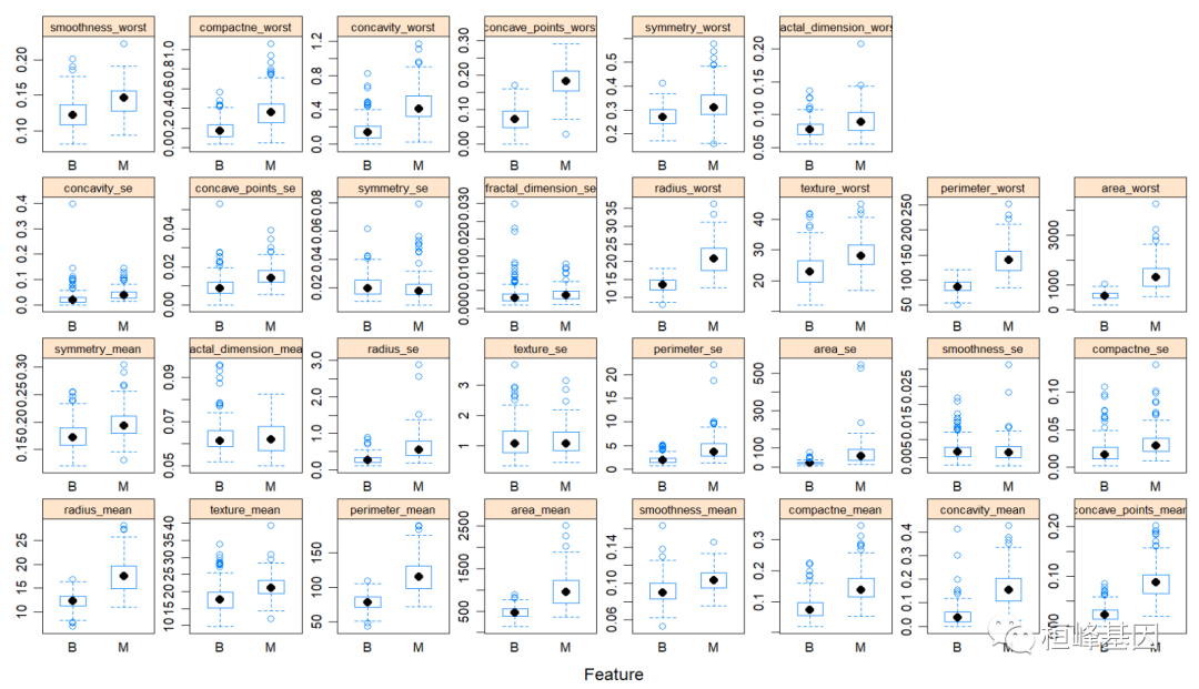
使用递归特征消去进行特征选择
set.seed(100)
options(warn = -1)

subsets <- c(1:5, 10, 15, 18)

ctrl <- rfeControl(functions = rfFuncs, method = "repeatedcv", repeats = 5, verbose = FALSE)

lmProfile <- rfe(x = trainData[, 2:31], y = trainData$diagnosis, sizes = subsets,
    rfeControl = ctrl)
head(lmProfile$results$Kappa)
## [1] 0.7378337 0.8313095 0.8704547 0.8650509 0.8678856 0.8987063
xyplot(lmProfile$results$Kappa ~ lmProfile$results$Variables, ylab = "Kappa", xlab = "Variables",
    type = c("g", "p", "l"), auto.key = TRUE)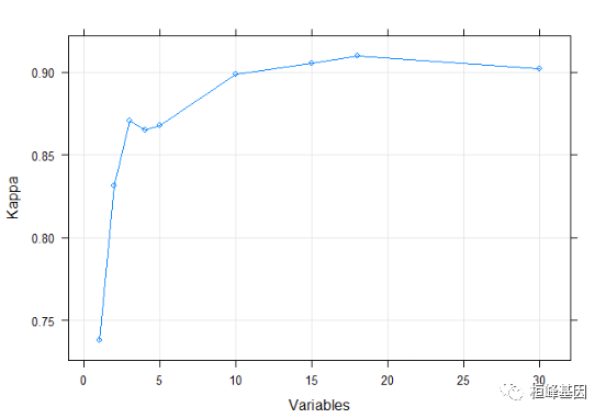
xyplot
xyplot(lmProfile$results$Accuracy ~ lmProfile$results$Variables, ylab = "Accuracy",
    xlab = "Variables", type = c("g", "p", "l"), auto.key = TRUE)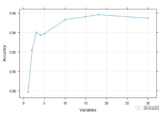
bwplot
bwplot(lmProfile$results$Accuracy ~ lmProfile$results$Variables, ylab = "Accuracy",
    xlab = "Variables", type = c("g", "p", "l"), auto.key = TRUE)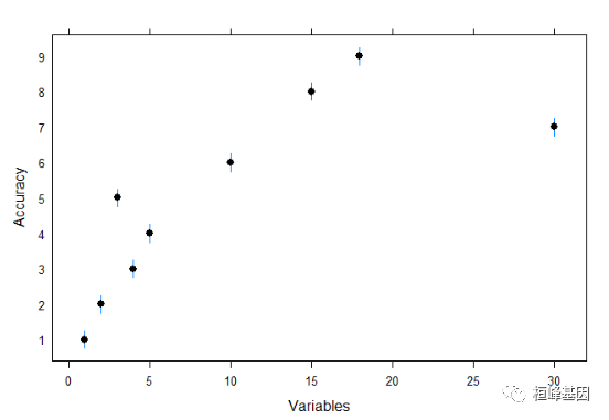
dotplot
dotplot(lmProfile$results$Accuracy ~ lmProfile$results$Variables, ylab = "Accuracy",
    xlab = "Variables", type = c("g", "p", "l"), auto.key = TRUE)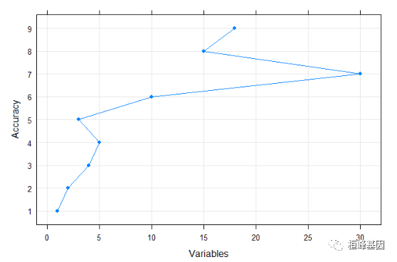
stripplot
stripplot(lmProfile$results$Accuracy ~ lmProfile$results$Variables, ylab = "Accuracy",
    xlab = "Variables", type = c("g", "p", "l"), auto.key = TRUE)
定义测试参数
# Define the training control
fitControl <- trainControl(
  method = 'cv',                   # k-fold cross validation
  number = 5,                      # number of folds
  savePredictions = 'final',       # saves predictions for optimal tuning parameter
  classProbs = T,                  # should class probabilities be returned
  summaryFunction=twoClassSummary  # results summary function
)
构建Adaboost分类器
model_adaboost = train(diagnosis ~ ., data = trainData, method = "adaboost", tuneLength = 2,
    trControl = fitControl)
model_adaboost
## AdaBoost Classification Trees
##
## 398 samples
##  30 predictor
##   2 classes: 'B', 'M'
##
## No pre-processing
## Resampling: Cross-Validated (5 fold)
## Summary of sample sizes: 319, 319, 318, 318, 318
## Resampling results across tuning parameters:
##
##   nIter  method         ROC        Sens   Spec
##    50    Adaboost.M1    0.9908414  0.980  0.9252874
##    50    Real adaboost  0.7658046  0.992  0.9252874
##   100    Adaboost.M1    0.9919310  0.980  0.9388506
##   100    Real adaboost  0.8226345  0.988  0.9252874
##
## ROC was used to select the optimal model using the largest value.
## The final values used for the model were nIter = 100 and method = Adaboost.M1.
plot(model_adaboost, main = "Adaboost")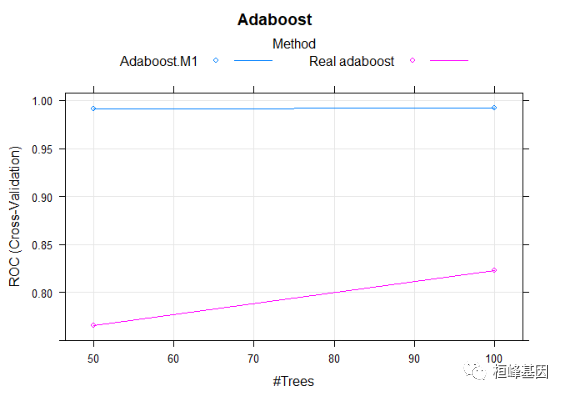
计算变量重要性
对于回归和分类模型的变量需要确定一下变量的重要性,我们可以看到BreastCancer的数据集里面自变量有30个,需要我们进一步筛选一下重要的变量,或者说决定性变量,去掉那些无关紧要可有可无的变量,减少计算复杂度以及后期可操作性。
varimp_mars <- varImp(model_adaboost)
plot(varimp_mars, main = "Variable Importance with BreastCancer")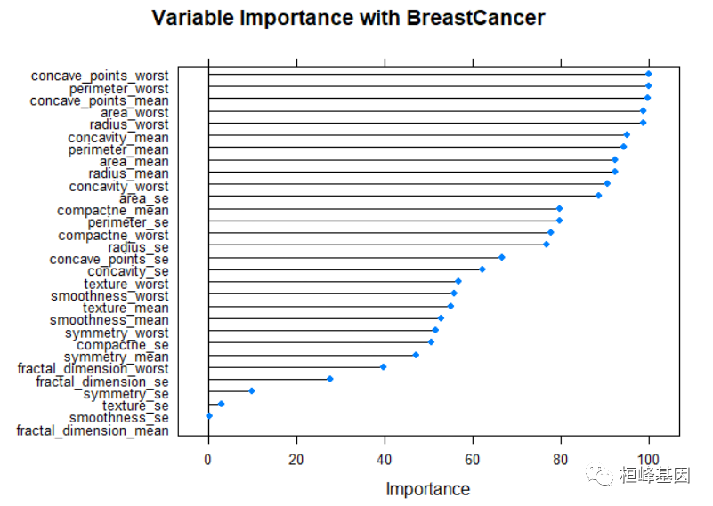
计算混淆矩阵
对于分类模型的只需要看混淆矩阵比较清晰的看出来分类的正确性。
predProb <- predict(model_adaboost, testData, type = "prob")
head(predProb)
##            B         M
## 1 0.02068105 0.9793190
## 2 0.19066233 0.8093377
## 3 0.43677815 0.5632219
## 4 0.03281830 0.9671817
## 5 0.17298856 0.8270114
## 6 0.05044144 0.9495586
predicted = predict(model_adaboost, testData)
testData$predProb = predProb$B
confusionMatrix(reference = testData$diagnosis, data = predicted, mode = "everything",
    positive = "B")
## Confusion Matrix and Statistics
##
##           Reference
## Prediction   B   M
##          B 104   2
##          M   3  61
##
##                Accuracy : 0.9706
##                  95% CI : (0.9327, 0.9904)
##     No Information Rate : 0.6294
##     P-Value [Acc > NIR] : <2e-16
##
##                   Kappa : 0.9372
##
##  Mcnemar's Test P-Value : 1
##
##             Sensitivity : 0.9720
##             Specificity : 0.9683
##          Pos Pred Value : 0.9811
##          Neg Pred Value : 0.9531
##               Precision : 0.9811
##                  Recall : 0.9720
##                      F1 : 0.9765
##              Prevalence : 0.6294
##          Detection Rate : 0.6118
##    Detection Prevalence : 0.6235
##       Balanced Accuracy : 0.9701
##
##        'Positive' Class : B
##
绘制ROC曲线
但是根据模型构建后需要进行准确性的评估我们就需要计算一下AUC,绘制ROC曲线来展示一下准确性。
library(ROCR)
pred = prediction(testData$predProb, testData$diagnosis)
perf = performance(pred, measure = "fpr", x.measure = "tpr")
plot(perf, lwd = 2, col = "blue", main = "ROC")
abline(a = 0, b = 1, col = 2, lwd = 1, lty = 2)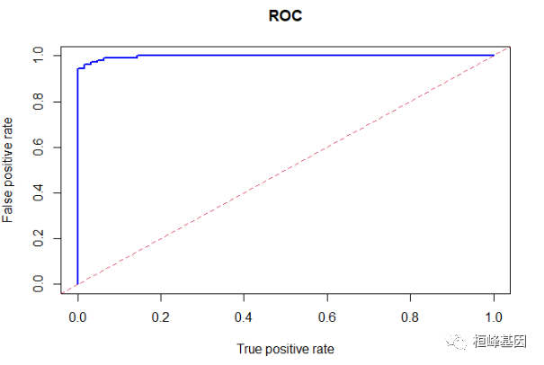
构建随机森林分类器
# Train the model using rf
model_rf = train(diagnosis ~ ., data = trainData, method = "rf", tuneLength = 5,
    trControl = fitControl)
model_rf
## Random Forest
##
## 398 samples
##  30 predictor
##   2 classes: 'B', 'M'
##
## No pre-processing
## Resampling: Cross-Validated (5 fold)
## Summary of sample sizes: 319, 318, 318, 318, 319
## Resampling results across tuning parameters:
##
##   mtry  ROC        Sens   Spec
##    2    0.9887034  0.984  0.9186207
##    9    0.9874598  0.976  0.9252874
##   16    0.9868000  0.976  0.9183908
##   23    0.9890690  0.964  0.9255172
##   30    0.9887448  0.960  0.9321839
##
## ROC was used to select the optimal model using the largest value.
## The final value used for the model was mtry = 23.
多个分类器比较
models_compare <- resamples(list(ADABOOST = model_adaboost, RF = model_rf))
summary(models_compare)
##
## Call:
## summary.resamples(object = models_compare)
##
## Models: ADABOOST, RF
## Number of resamples: 5
##
## ROC
##               Min.   1st Qu.    Median     Mean   3rd Qu.      Max. NA's
## ADABOOST 0.9793103 0.9903448 0.9940000 0.991931 0.9980000 0.9980000    0
## RF       0.9763333 0.9810345 0.9893333 0.989069 0.9993103 0.9993333    0
##
## Sens
##          Min. 1st Qu. Median  Mean 3rd Qu. Max. NA's
## ADABOOST 0.94    0.96   1.00 0.980    1.00    1    0
## RF       0.88    0.98   0.98 0.964    0.98    1    0
##
## Spec
##               Min. 1st Qu.    Median      Mean   3rd Qu.      Max. NA's
## ADABOOST 0.8965517     0.9 0.9310345 0.9388506 0.9666667 1.0000000    0
## RF       0.8965517     0.9 0.9310345 0.9255172 0.9333333 0.9666667    0
# Draw box plots to compare models
scales <- list(x = list(relation = "free"), y = list(relation = "free"))
bwplot(models_compare, scales = scales)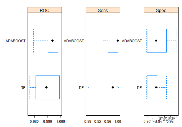
fastAdaboost实现
test_adaboost <- adaboost(diagnosis ~ ., trainData, 10)
pred <- predict(test_adaboost, newdata = testData)
print(pred$error)
## [1] 0.03529412
adabag实现
library(adabag)
model_adabag <- boosting(diagnosis ~ ., data = trainData, mfinal = 10, boos = TRUE)
Freq <- table(trainData$diagnosis, model_adabag$class)
head(Freq)
##
##       B   M
##   B 250   0
##   M   0 148
model_error <- errorevol(model_adabag, trainData)
model_error_data <- data.frame(model_error$error, subsets = 1:10)
head(model_error_data)
##   model_error.error subsets
## 1       0.045226131       1
## 2       0.045226131       2
## 3       0.020100503       3
## 4       0.005025126       4
## 5       0.000000000       5
## 6       0.000000000       6
library(rCharts)
nPlot(model_error.error~subsets,data=model_error_data,type='lineChart')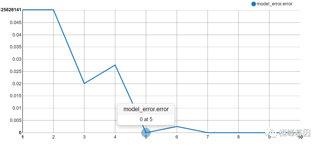
Reference
Zhu, Ji, et al. “Multi-class adaboost” Ann Arbor 1001.48109 (2006): 1612.
Freund, Y. and Schapire, R.E. (1996):“Experiments with a new boosting algorithm” . In Proceedings of the Thirteenth International Conference on Machine Learning, pp. 148–156, Morgan Kaufmann.
Fits the AdaBoost.M1 (Freund and Schapire, 1996) and SAMME (Zhu et al., 2009) algorithms using classification trees as single classifiers.
号外号外,桓峰基因单细胞生信分析免费培训课程即将开始快来报名吧!
桓峰基因,铸造成功的您!
未来桓峰基因公众号将不间断的推出单细胞系列生信分析教程,
敬请期待!!
桓峰基因官网正式上线,请大家多多关注,还有很多不足之处,大家多多指正!http://www.kyohogene.com/
桓峰基因和投必得合作,文章润色优惠85折,需要文章润色的老师可以直接到网站输入领取桓峰基因专属优惠券码:KYOHOGENE,然后上传,付款时选择桓峰基因优惠券即可享受85折优惠哦!https://www.topeditsci.com/


 6579
6579


 被折叠的 条评论
为什么被折叠?
被折叠的 条评论
为什么被折叠?
 到【灌水乐园】发言


