MachineLearning 37. 机器学习之倾斜随机生存森林 (obliqueRSF)-CSDN博客

本文链接：https://blog.csdn.net/weixin_41368414/article/details/139457437

简介

斜随机生存森林(ORSF)是一种集成方法，用于右删节存活数据，它使用输入变量的线性组合递归地划分一组训练数据。正则化Cox比例风险模型用于识别每个递归划分步骤中输入变量的线性组合。模拟和真实数据的基准测试结果表明，与随机生存森林、条件推理森林、回归和增强相比，ORSF预测的风险函数具有较高的预测价值。在Jackson心脏研究数据的应用中，使用ORSF证明了变量和部分依赖性，并强调了其10年预测动脉粥样硬化性心血管疾病事件(ASCVD;中风，冠心病)。根据ORSF、条件推理森林和合并队列风险方程，展示了比较变量和部分效应估计的可视化效果。

软件包安装

软件包安装两种方式：

install.packages("devtools")
install.packages("remotes")
remotes::install_github("ropensci/aorsf")
install.packages('aorsf')

数据读取

数据集来自survival包中的pbc,来自梅奥诊所在1974年至1984年间进行的PBC试验。在这10年期间，共有424名PBC患者转至梅奥诊所，符合D-青霉胺随机安慰剂对照试验的资格标准。数据集中的前312例患者参加了随机试验，数据基本完整。另外112例患者没有参加临床试验，但同意记录基本测量值并随访以维持生存。其中6例在诊断后不久就失去了随访，所以这里的数据是额外的106例病例以及312名随机参与者。

age: in years
albumin: serum albumin (g/dl)
alk.phos: alkaline phosphotase (U/liter)
ascites: presence of ascites
ast: aspartate aminotransferase, once called SGOT (U/ml)
bili: serum bilirunbin (mg/dl)
chol: serum cholesterol (mg/dl)
copper: urine copper (ug/day)
edema: 0 no edema, 0.5 untreated or successfully treated 1 edema despite diuretic therapy
hepato: presence of hepatomegaly or enlarged liver
id: case number
platelet: platelet count
protime: standardised blood clotting time
sex: m/f
spiders: blood vessel malformations in the skin
stage: histologic stage of disease (needs biopsy)
status: status at endpoint, 0/1/2 for censored, transplant, dead
time: number of days between registration and the earlier of death,transplantion, or study analysis in July, 1986
trt: 1/2/NA for D-penicillmain, placebo, not randomised
trig: triglycerides (mg/dl)

library(aorsf)
library(tidyverse)

pbc <- pbc_orsf
# An oblique survival RF
head(pbc)
##   id time status             trt      age sex ascites hepato spiders edema bili
## 1  1  400      1 d_penicill_main 58.76523   f       1      1       1     1 14.5
## 2  2 4500      0 d_penicill_main 56.44627   f       0      1       1     0  1.1
## 3  3 1012      1 d_penicill_main 70.07255   m       0      0       0   0.5  1.4
## 4  4 1925      1 d_penicill_main 54.74059   f       0      1       1   0.5  1.8
## 5  5 1504      0         placebo 38.10541   f       0      1       1     0  3.4
## 7  7 1832      0         placebo 55.53457   f       0      1       0     0  1.0
##   chol albumin copper alk.phos    ast trig platelet protime stage
## 1  261    2.60    156   1718.0 137.95  172      190    12.2     4
## 2  302    4.14     54   7394.8 113.52   88      221    10.6     3
## 3  176    3.48    210    516.0  96.10   55      151    12.0     4
## 4  244    2.54     64   6121.8  60.63   92      183    10.3     4
## 5  279    3.53    143    671.0 113.15   72      136    10.9     3
## 7  322    4.09     52    824.0  60.45  213      204     9.7     3

pbc = na.omit(pbc)
table(pbc$status)
## 
##   0   1 
## 165 111

library(sampling)
set.seed(123)
# 每层抽取70%的数据
train_id <- strata(pbc, "status", size = rev(round(table(pbc$status) * 0.7)))$ID_unit
# 训练数据
trainData <- pbc[train_id, ]
# 测试数据
testData <- pbc[-train_id, ]

实例操作

构建模型

pbc_fit <- orsf(data = trainData, n_tree = 20, formula = Surv(time, status) ~ . -
    id)
res <- orsf_summarize_uni(pbc_fit)
library(data.table)
head(as.data.table(res))
##    variable importance  value      mean      medn        lwr       upr
##      <char>      <num> <char>     <num>     <num>      <num>     <num>
## 1:     bili  0.5172414   0.60 0.2663037 0.1932877 0.05741174 0.4269579
## 2:     bili  0.5172414   0.80 0.2724312 0.1996642 0.06232726 0.4480355
## 3:     bili  0.5172414   1.60 0.3080398 0.2189249 0.08703489 0.5017554
## 4:     bili  0.5172414   3.70 0.4404167 0.3980655 0.20825906 0.6614583
## 5:     bili  0.5172414   7.18 0.5075947 0.5301124 0.28791330 0.7291667
## 6:   copper  0.4909091   27.2 0.2997513 0.2107370 0.06277056 0.5096297
##    pred_horizon  level
##           <num> <char>
## 1:         1741   <NA>
## 2:         1741   <NA>
## 3:         1741   <NA>
## 4:         1741   <NA>
## 5:         1741   <NA>
## 6:         1741   <NA>

验证

预测predict()参数中pred_type有7种选择：none, surv, risk, chf, mort, leaf, or time, 可以获得预测生存矩阵和相对风险：

# predicted risk, the default
predict(pbc_fit, new_data = testData, pred_type = "risk", pred_horizon = c(360, 720,
    1800))
# predicted survival, i.e., 1 - risk
predict(pbc_fit, new_data = testData, pred_type = "surv", pred_horizon = c(360, 720,
    1800))
# predicted cumulative hazard function (expected number of events for person i
# at time j)
predict(pbc_fit, new_data = testData, pred_type = "chf", pred_horizon = c(360, 720,
    1800))
# Predict mortality
predict(pbc_fit, new_data = testData, pred_type = "mort")

变量重要性

针对变量分析包括：

变量的重要性（Variable Importance）；
变量的选择（Variable selection）；
变量的互作（Variable Interactions）。

# Variable Importance
orsf_vi(pbc_fit)
##       bili     copper    ascites      edema        age    protime    albumin 
## 0.51724138 0.49090909 0.47222222 0.36834823 0.34545455 0.32075472 0.24444444 
##        ast   platelet     hepato       trig       chol      stage    spiders 
## 0.17741935 0.15873016 0.14583333 0.14285714 0.14285714 0.13235294 0.09803922 
##        sex   alk.phos        trt 
## 0.06818182 0.05263158 0.00000000

# Variable selection
orsf_vs(pbc_fit, n_predictor_min = 5)
##     n_predictors stat_value                        variables_included
##            <int>      <num>                                    <list>
##  1:            5  0.8560700     age,ascites,bili,copper,edema,protime
##  2:            6  0.8484568    age,ascites,bili,chol,copper,edema,...
##  3:            7  0.8381687  age,albumin,ascites,bili,chol,copper,...
##  4:            8  0.8504115  age,albumin,ascites,bili,chol,copper,...
##  5:            9  0.8565844  age,albumin,ascites,bili,chol,copper,...
##  6:           10  0.8525720  age,albumin,ascites,bili,chol,copper,...
##  7:           11  0.8614198     age,albumin,ascites,ast,bili,chol,...
##  8:           12  0.8702675     age,albumin,ascites,ast,bili,chol,...
##  9:           13  0.8534979 age,albumin,alk.phos,ascites,ast,bili,...
## 10:           14  0.8308642 age,albumin,alk.phos,ascites,ast,bili,...
## 11:           15  0.8565844 age,albumin,alk.phos,ascites,ast,bili,...
## 12:           16  0.8412551 age,albumin,alk.phos,ascites,ast,bili,...
## 13:           17  0.8493827 age,albumin,alk.phos,ascites,ast,bili,...
##                                        predictors_included predictor_dropped
##                                                     <list>            <char>
##  1:              age,ascites_1,edema_1,bili,copper,protime           protime
##  2:             age,ascites_1,edema_1,bili,chol,copper,...              chol
##  3:            age,ascites_1,edema_1,bili,chol,albumin,...           albumin
##  4:          age,ascites_1,spiders_1,edema_1,bili,chol,...         spiders_1
##  5:          age,ascites_1,spiders_1,edema_1,bili,chol,...              trig
##  6:          age,ascites_1,spiders_1,edema_1,bili,chol,...             stage
##  7:          age,ascites_1,spiders_1,edema_1,bili,chol,...               ast
##  8:          age,ascites_1,spiders_1,edema_1,bili,chol,...          platelet
##  9:          age,ascites_1,spiders_1,edema_1,bili,chol,...          alk.phos
## 10:      age,ascites_1,hepato_1,spiders_1,edema_1,bili,...          hepato_1
## 11: age,ascites_1,hepato_1,spiders_1,edema_0.5,edema_1,...         edema_0.5
## 12:   age,sex_f,ascites_1,hepato_1,spiders_1,edema_0.5,...             sex_f
## 13: trt_placebo,age,sex_f,ascites_1,hepato_1,spiders_1,...       trt_placebo

# Variable Interactions
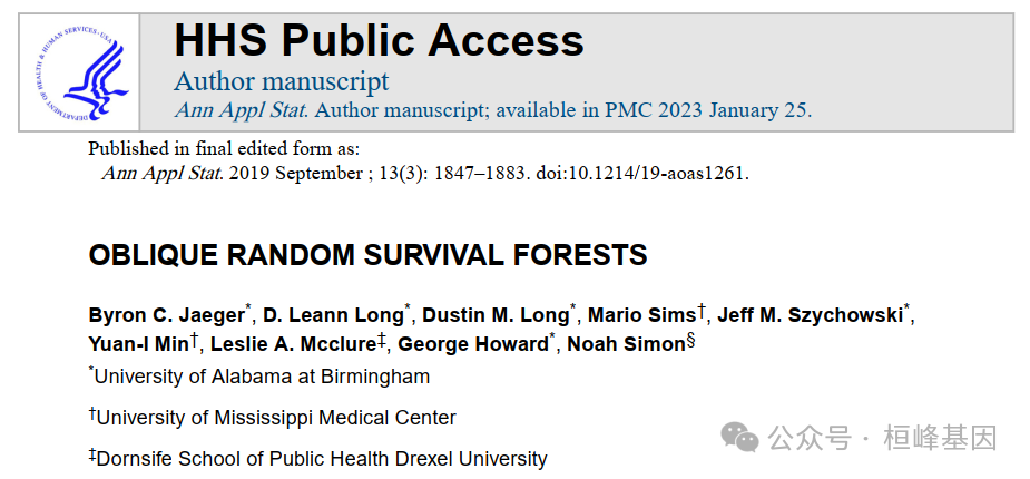
interaction <- as.data.frame(orsf_vint(pbc_fit)[, 1:2])
interaction = interaction %>%
    separate_wider_delim(interaction, "..", names = c("V1", "V2"))
head(interaction)
## # A tibble: 6 × 3
##   V1      V2      score
##   <chr>   <chr>   <dbl>
## 1 ascites edema    2.76
## 2 ascites bili     1.89
## 3 ascites spiders  1.88
## 4 bili    stage    1.67
## 5 edema   stage    1.53
## 6 edema   copper   1.52

ggplot(interaction) + geom_point(aes(x = V1, y = V2, color = score, size = score)) +
    theme_bw() + labs(y = "", x = "") + theme(axis.text.x = element_text(angle = 90,
    vjust = 1, hjust = 1))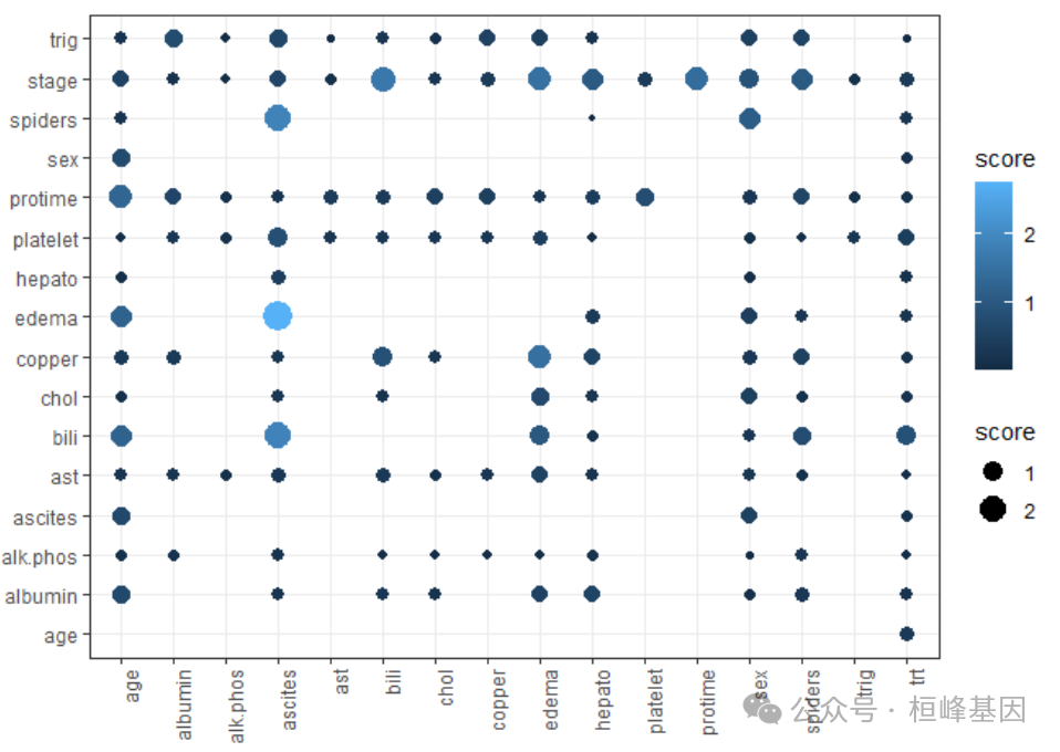

一致性

library(survival)
# 生存分析
pred <- predict(pbc_fit, testData, pred_type = "surv")
str(pred)
##  num [1:83, 1] 0.0197 0.3874 0.7159 0.64 0.8972 ...

p <- predict(pbc_fit, new_data = testData, pred_type = "risk", pred_horizon = c(360,
    720, 1800))
testData$pred = pred
C_index <- data.frame(Cindex = as.numeric(summary(coxph(Surv(time, status) ~ pred,
    testData))$concordance[1]))
C_index
##      Cindex
## 1 0.7800128

生存分析

根据风险值我们可以将患者分为高低风险组，然后绘制生存曲线：

library(survminer)
testData$risk = p[, 1]
group = ifelse(testData$risk > mean(testData$risk), "High", "Low")
f <- survfit(Surv(testData$time, testData$status) ~ group)
f
## Call: survfit(formula = Surv(testData$time, testData$status) ~ group)
## 
##             n events median 0.95LCL 0.95UCL
## group=High 20     16   1191     611      NA
## group=Low  63     17   3839    3086      NA

ggsurvplot(f, data = testData, surv.median.line = "hv", legend.title = "Risk Group",
    legend.labs = c("Low Risk", "High Risk"), pval = TRUE, ggtheme = theme_bw())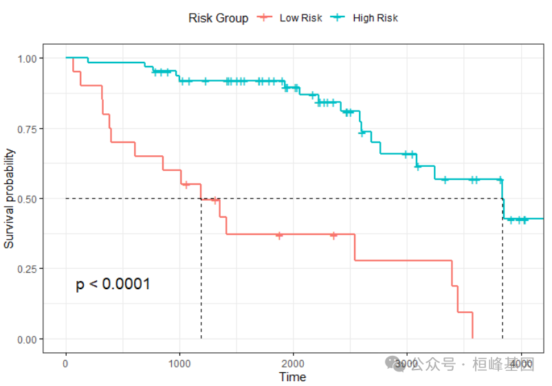

绘制ROC曲线

由于我们所作的模型根时间密切相关因此我们选择timeROC,可以快速的技术出来不同时期的ROC，进一步作图：

library(timeROC)
res <- timeROC(T = testData$time, delta = testData$status, marker = testData$risk,
    cause = 1, weighting = "marginal", times = c(360, 720, 1800), ROC = TRUE, iid = TRUE)
res$AUC
##     t=360     t=720    t=1800 
## 0.7961538 0.8581081 0.8590447

confint(res, level = 0.95)$CI_AUC
##         2.5%  97.5%
## t=360  55.39 103.84
## t=720  70.96 100.66
## t=1800 74.68  97.13

plot(res, time = 360, col = "red", title = FALSE, lwd = 2)
plot(res, time = 720, add = TRUE, col = "blue", lwd = 2)
plot(res, time = 1800, add = TRUE, col = "green", lwd = 2)
legend("bottomright", c(paste("1 Years ", round(res$AUC[1], 2)), paste("2 Years ",
    round(res$AUC[2], 2)), paste("5 Years ", round(res$AUC[3], 2))), col = c("red",
    "blue", "green"), lty = 1, lwd = 2)

不同时间节点的AUC曲线及其置信区间

再分析不同时间节点的AUC曲线及其置信区间，由于数据量非常小，此图并不明显。

plotAUCcurve(res, conf.int = TRUE, col = "red")

Reference

Jaeger BC, Long DL, Long DM, Sims M, Szychowski JM, Min Y, Mcclure LA, Howard G, Simon N (2019). “Oblique random survival forests.” The Annals of Applied Statistics, 13(3). doi:10.1214/19-aoas1261 https://doi.org/10.1214/19-aoas1261.
Jaeger BC, Welden S, Lenoir K, Speiser JL, Segar MW, Pandey A, Pajewski NM (2023). “Accelerated and interpretable oblique random survival forests.” Journal of Computational and Graphical Statistics, 1-16. doi:10.1080/10618600.2023.2231048 https://doi.org/10.1080/10618600.2023.2231048.
Horst AM, Hill AP, Gorman KB (2020). palmerpenguins: Palmer Archipelago (Antarctica) penguin data. R package version 0.1.0, https://allisonhorst.github.io/palmerpenguins/.
Menze, H B, Kelm, Michael B, Splitthoff, N D, Koethe, Ullrich, Hamprecht, A F (2011). “On oblique random forests.” In Machine Learning and Knowledge Discovery in Databases: European Conference, ECML PKDD 2011, Athens, Greece, September 5-9, 2011, Proceedings, Part II 22, 453-469. Springer. Greenwell, M B, Boehmke, C B, McCarthy, J A (2018). “A simple and effective model-based variable importance measure.” arXiv preprint arXiv:1805.04755.