


简 介
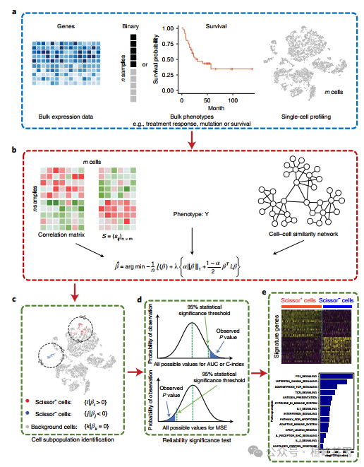
单细胞RNA测序(scRNA-seq)在异质组织中区分细胞类型、状态和谱系。然而,目前的单细胞数据不能直接将细胞簇与特定表型联系起来。在这里,我们提出Scissor方法,从单细胞数据中识别与给定表型相关的细胞亚群。Scissor通过首先量化每个单细胞和每个大样本之间的相似性,整合了表型相关的大样本表达数据和单细胞数据。然后,优化了与样本表型相关矩阵的回归模型,以确定相关的亚群。将Scissor应用于肺癌scRNA-seq数据集,确定了与生存率较差 和TP53突变相关的细胞亚群。在黑色素瘤中,Scissor发现了与免疫治疗反应相关的低PDCD1/CTLA4和高TCF7表达的T细胞亚群。除癌症外,Scissor在解释面部肩胛骨肌肉萎缩症和阿尔茨海默病数据集方面也很有效。Scissor通过利用表型和大体积组学数据集,从单细胞分析中识别生物学和临床相关的细胞亚群。
Sicssor包含拟议的Sicssor算法(Sicssor功能),这是一种新的单细胞数据分析方法,利用大量表型从单细胞测序数据中识别最高度表型相关的细胞亚群。Sicssor的优势可以简单概括如下:
首先,通过Sicssor识别的表型相关细胞具有独特的分子特性,涉及到关键的标记基因和给定表型的生物学过程。
其次,Scissor不需要对单细胞数据进行任何无监督聚类,从而避免了对细胞簇数或聚类分辨率的主观决定。
最后,Scissor提供了一个灵活的框架来整合大量数据中的各种外部表型,以指导单细胞数据分析,从而实现临床和生物学相关细胞亚群的无假设鉴定。
软件包安装
软件包安装非常简单,
if(!require(Scissor))
  devtools::install_github('sunduanchen/Scissor')
但是要注意以下里面依赖的Seurat软件包,因为我安装的是V5+版的,所以在读取对象的时候显示Assay5,因此需要object的class 为 Assay,按照如下代码加入options()。
library(Scissor)library(Seurat)
options(Seurat.object.assay.version = "v3")数据读取
Scissor输入有三个数据源:单细胞表达矩阵、批量表达矩阵和感兴趣的表型。每个大样本的表型注释可以是一个连续的因变量,二元组指标载体,或临床生存数据。我们使用肺腺癌(LUAD) scRNA-seq癌细胞的几个应用数据作为示例来展示如何在实际应用中执行Scissor。
数据源需要三种类型数据:
单细胞数据:count矩阵或者Seurat创建的object;
bulk转录组数据:表达矩阵
临床信息数据:cox回归要求必须有time和status,其他两种不需要
看下例子中的数据格式:
1. 单细胞数据:
准备原始count矩阵,如下:
location <- "https://xialab.s3-us-west-2.amazonaws.com/Duanchen/Scissor_data/"
load(url(paste0(location, 'scRNA-seq.RData')))
dim(sc_dataset)
## [1] 33694 4102class(sc_dataset)## [1] "matrix" "array"利用Seurat_preprocessing()对原始矩阵进行处理,包括"RNA"、"RNA_nn"、"RNA_snn"、"pca"、"tsne"、"umap"。详细流程如下:
Create a Seurat object from raw data.
Normalize the count data present in a given assay.
Identify the variable features.
Scales and centers features in the dataset.
Run a PCA dimensionality reduction.
Constructs a Shared Nearest Neighbor (SNN) Graph for a given dataset.
Identify clusters of cells by a shared nearest neighbor (SNN) modularity optimization based clustering algorithm.
Run t-distributed Stochastic Neighbor Embedding (t-SNE) dimensionality reduction on selected features.
Runs the Uniform Manifold Approximation and Projection (UMAP) dimensional reduction technique.
sc_dataset <- Seurat_preprocessing(sc_dataset, verbose = F)## Warning: The default method for RunUMAP has changed from calling Python UMAP via reticulate to the R-native UWOT using the cosine metric
## To use Python UMAP via reticulate, set umap.method to 'umap-learn' and metric to 'correlation'
## This message will be shown once per sessionnames(sc_dataset)## [1] "RNA" "RNA_nn" "RNA_snn" "pca" "tsne" "umap"DimPlot(sc_dataset, reduction = 'umap', label = T, label.size = 10)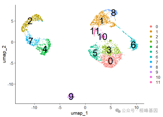
2. bulk转录组数据
load(url(paste0(location, 'TCGA_LUAD_exp1.RData')))
dim(bulk_dataset)
## [1] 56716 471bulk_dataset[1:5,1:5]## TCGA-05-4249 TCGA-05-4250 TCGA-05-4382 TCGA-05-4384 TCGA-05-4389
## TSPAN6 57.523977 66.4940573 30.905120 35.104344 107.71744400
## TNMD 0.000000 0.1748819 0.000000 0.000000 0.03309504
## DPM1 98.838134 135.2046911 84.362971 89.105535 98.17846534
## SCYL3 16.233391 6.0050820 6.226792 16.930497 9.97072687
## C1orf112 5.139334 7.4082268 4.778406 4.139623 7.599101563. 临床信息数据
a) 临床生存数据
load(url(paste0(location, 'TCGA_LUAD_survival.RData')))
dim(bulk_survival)
## [1] 471 3head(bulk_survival)## TCGA_patient_barcode OS_time Status
## 1 TCGA-05-4249 1158 0
## 2 TCGA-05-4250 121 1
## 3 TCGA-05-4382 607 0
## 4 TCGA-05-4384 426 0
## 5 TCGA-05-4389 1369 0
## 6 TCGA-05-4390 1126 0all(colnames(bulk_dataset) == bulk_survival$TCGA_patient_barcode)## [1] TRUEphenotype <- bulk_survival[,2:3]
colnames(phenotype) <- c("time", "status")
head(phenotype)## time status
## 1 1158 0
## 2 121 1
## 3 607 0
## 4 426 0
## 5 1369 0
## 6 1126 0实例操作
Scissor可以支持三种模型的构建,一种是Cox回归模型,一种是logistic回归模型,另一种是gaussian模型。由family = c("gaussian", "binomial", "cox"),参数控制模型算法:
Scissor(
  bulk_dataset,
  sc_dataset,
  phenotype,
  tag = NULL,
  alpha = NULL,
  cutoff = 0.2,
  family = c("gaussian", "binomial", "cox"),
  Save_file = "Scissor_inputs.RData",
  Load_file = NULL
)
Scissor应用与Cox回归模型
1) 执行Scissor()选择表型相关细胞
执行Scissor()选择表型相关的细胞亚群。
infos1 <- Scissor(bulk_dataset,
                  sc_dataset,
                  phenotype,
                  alpha = 0.05,
                  family = "cox",
                  Save_file = 'Scissor_LUAD_survival.RData')
## [1] "|**************************************************|"
## [1] "Performing quality-check for the correlations"
## [1] "The five-number summary of correlations:"
## 0% 25% 50% 75% 100%
## 0.01319134 0.19658357 0.23945759 0.29808510 0.83727807
## [1] "|**************************************************|"
## [1] "Perform cox regression on the given clinical outcomes:"
## [1] "alpha = 0.05"
## [1] "Scissor identified 201 Scissor+ cells and 4 Scissor- cells."
## [1] "The percentage of selected cell is: 4.998%"
## [1] "|**************************************************|"总的来说,Scissor鉴定出201个与较差存活率相关的Scissor+cells和4个与良好存活率相关的Scissor- cells。这些选定的细胞占总数4102个细胞的5%。通过在Seurat对象sc_dataset中添加一个新的注释来可视化Scissor选择的细胞。
names(infos1)## [1] "para" "Coefs" "Scissor_pos" "Scissor_neg"length(infos1$Scissor_pos)## [1] 201infos1$Scissor_pos[1:4]## [1] "AAAGTAGAGGAGCGAG_19" "AACCATGCATCTCCCA_19" "AACCGCGAGCTGCGAA_20"
## [4] "AACTCAGTCCGCGGTA_19"length(infos1$Scissor_neg)## [1] 4infos1$Scissor_neg## [1] "ACGCCAGTCCTCCTAG_20" "ACGGGCTAGTGGCACA_20" "CCGGTAGGTACCCAAT_15"
## [4] "GACGCGTAGTGGTCCC_20"Scissor_select <- rep(0, ncol(sc_dataset))
names(Scissor_select) <- colnames(sc_dataset)
Scissor_select[infos1$Scissor_pos] <- 1
Scissor_select[infos1$Scissor_neg] <- 2
sc_dataset <- AddMetaData(sc_dataset, metadata = Scissor_select, col.name = "scissor")
infos1$para## $alpha
## [1] 0.05
##
## $lambda
## [1] 0.04229243
##
## $family
## [1] "cox"DimPlot(sc_dataset, reduction = 'umap', group.by = 'scissor', cols = c('grey','indianred1','royalblue'), pt.size = 1.2, order = c(2,1))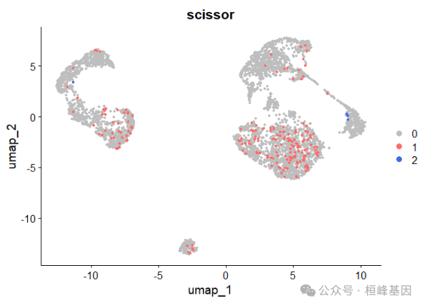
2) 调整模型参数
在上述实现中,我们将参数α设置为0.05 (alpha = 0.05)。参数α平衡l1规范和基于网络的惩罚的效果。较大的α倾向于强调l1规范以鼓励稀疏性,使得Scissor选择的细胞比使用较小α的结果少。
##Tune model paramters
infos2 <- Scissor(bulk_dataset,
                  sc_dataset,
                  phenotype,
                  alpha = NULL,
                  cutoff = 0.03,
                  family = "cox",
                  Load_file = 'Scissor_LUAD_survival.RData')
## [1] "alpha = 0.005"
## [1] "Scissor identified 887 Scissor+ cells and 28 Scissor- cells."
## [1] "The percentage of selected cell is: 22.306%"
##
## [1] "alpha = 0.01"
## [1] "Scissor identified 573 Scissor+ cells and 20 Scissor- cells."
## [1] "The percentage of selected cell is: 14.456%"
##
## [1] "alpha = 0.05"
## [1] "Scissor identified 201 Scissor+ cells and 4 Scissor- cells."
## [1] "The percentage of selected cell is: 4.998%"
##
## [1] "alpha = 0.1"
## [1] "Scissor identified 139 Scissor+ cells and 5 Scissor- cells."
## [1] "The percentage of selected cell is: 3.510%"
##
## [1] "alpha = 0.2"
## [1] "Scissor identified 78 Scissor+ cells and 5 Scissor- cells."
## [1] "The percentage of selected cell is: 2.023%"
## [1] "|**************************************************|"在上面的实现中,我们设置了一个新的百分比截断(cutoff = 0.03),当所选细胞的总百分比小于3%时,停止α搜索。对应的α = 0.2,选择了78个Scissor+ cells和5个Scissor- cells。为了避免在实际应用中任意选择alpha,建议根据所选细胞在总细胞中的百分比来搜索α。cut的默认值为0.2,即Scissor选择的细胞数量不应超过单个细胞数据中总细胞的20%。此外,用户可以设置自定义的α序列和百分比截止,以实现不同的目标
infos3 <- Scissor(bulk_dataset,
                  sc_dataset,
                  phenotype,
                  alpha = seq(1,10,2)/1000,
                  cutoff = 0.2,
                  family = "cox",
                  Load_file = 'Scissor_LUAD_survival.RData')
## [1] "alpha = 0.001"
## [1] "Scissor identified 1663 Scissor+ cells and 1870 Scissor- cells."
## [1] "The percentage of selected cell is: 86.129%"
##
## [1] "alpha = 0.003"
## [1] "Scissor identified 1264 Scissor+ cells and 37 Scissor- cells."
## [1] "The percentage of selected cell is: 31.716%"
##
## [1] "alpha = 0.005"
## [1] "Scissor identified 887 Scissor+ cells and 28 Scissor- cells."
## [1] "The percentage of selected cell is: 22.306%"
##
## [1] "alpha = 0.007"
## [1] "Scissor identified 729 Scissor+ cells and 24 Scissor- cells."
## [1] "The percentage of selected cell is: 18.357%"
## [1] "|**************************************************|"Scissor应用与logistic回归模型
b) 二元分类数据
load(url(paste0(location, 'TCGA_LUAD_TP53_mutation.RData')))
table(TP53_mutation)
## TP53_mutation
## 0 1
## 243 255###Execute Scissor to select the informative cells
phenotype <- TP53_mutation
tag <- c('wild-type', 'TP53 mutant')在另一个例子中,使用TCGA-LUAD提供的其他表型特征来指导鉴定相同的4,102个癌细胞中的细胞亚群。在这里,我们关注TP53,在人类恶性肿瘤中发现的最常见的突变肿瘤抑制基因之一。
##Prepare the bulk data and phenotype
load(url(paste0(location, 'TCGA_LUAD_exp2.RData')))
load(url(paste0(location, 'TCGA_LUAD_TP53_mutation.RData')))
table(TP53_mutation)
## TP53_mutation
## 0 1
## 243 255###Execute Scissor to select the informative cells
phenotype <- TP53_mutation
tag <- c('wild-type', 'TP53 mutant')
infos4 <- Scissor(bulk_dataset, sc_dataset, phenotype, tag = tag, alpha = 0.5,
family = "binomial", Save_file = "Scissor_LUAD_TP53_mutation.RData")## [1] "|**************************************************|"
## [1] "Performing quality-check for the correlations"
## [1] "The five-number summary of correlations:"
## 0% 25% 50% 75% 100%
## 0.01308976 0.19502200 0.23725380 0.29589213 0.83830571
## [1] "|**************************************************|"
## [1] "Current phenotype contains 243 wild-type and 255 TP53 mutant samples."
## [1] "Perform logistic regression on the given phenotypes:"
## [1] "alpha = 0.5"
## [1] "Scissor identified 173 Scissor+ cells and 160 Scissor- cells."
## [1] "The percentage of selected cell is: 8.118%"
## [1] "|**************************************************|"infos5 <- Scissor(bulk_dataset, sc_dataset, phenotype, tag = tag, alpha = 0.2,
family = "binomial", Load_file = "Scissor_LUAD_TP53_mutation.RData")## [1] "alpha = 0.2"
## [1] "Scissor identified 414 Scissor+ cells and 320 Scissor- cells."
## [1] "The percentage of selected cell is: 17.894%"
## [1] "|**************************************************|"Scissor_select <- rep(0, ncol(sc_dataset))
names(Scissor_select) <- colnames(sc_dataset)
Scissor_select[infos5$Scissor_pos] <- 1
Scissor_select[infos5$Scissor_neg] <- 2
sc_dataset <- AddMetaData(sc_dataset, metadata = Scissor_select, col.name = "scissor")
DimPlot(sc_dataset, reduction = 'umap', group.by = 'scissor', cols = c('grey','indianred1','royalblue'), pt.size = 1.2, order = c(2,1))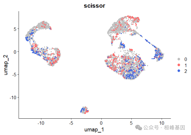
可靠性显著性检验
为了确定推断的表型-细胞关联是否可靠,我们使用功能可靠性。检验进行信度显著性检验。可靠性显著性检验的动机是:如果选择的单细胞和批量数据不适合表型与细胞之间的关联,则相关性的信息量会减少,并且与表型标签不太相关。因此,相应的预测性能会很差,并且与随机排列的标签没有明显的区别。
load('Scissor_LUAD_survival.RData')
numbers <- length(infos1$Scissor_pos) + length(infos1$Scissor_neg)
result1 <- reliability.test(X, Y, network, alpha = 0.05, family = "cox", cell_num = numbers, n = 10, nfold = 10)
## Warning: 程辑包'progress'是用R版本4.3.2 来建造的## Warning: 程辑包'survival'是用R版本4.3.3 来建造的## [1] "|**************************************************|"
## [1] "Perform cross-validation on X with true label"
## Finished!
## [1] "|**************************************************|"
## [1] "Perform cross-validation on X with permutated label"
## Finished!
## [1] "Test statistic = 0.628"
## [1] "Reliability significance test p = 0.000"names(result1)## [1] "statistic" "p" "c_index_test_real"
## [4] "c_index_test_back"load('Scissor_LUAD_TP53_mutation.RData')
numbers <- length(infos5$Scissor_pos) + length(infos5$Scissor_neg)
result2 <- reliability.test(X, Y, network, alpha = 0.2, family = "binomial", cell_num = numbers, n = 10, nfold = 10)## Warning: 程辑包'pROC'是用R版本4.3.2 来建造的## Type 'citation("pROC")' for a citation.##
## 载入程辑包:'pROC'## The following objects are masked from 'package:stats':
##
## cov, smooth, var## [1] "|**************************************************|"
## [1] "Perform cross-validation on X with true label"
## Finished!
## [1] "|**************************************************|"
## [1] "Perform cross-validation on X with permutated label"
## Finished!
## [1] "Test statistic = 0.790"
## [1] "Reliability significance test p = 0.000"names(result2)## [1] "statistic" "p" "AUC_test_real" "AUC_test_back"result2## $statistic
## [1] 0.7900128
##
## $p
## [1] 0
##
## $AUC_test_real
## [1] 0.8184615 0.8366667 0.8028846 0.8000000 0.8107692 0.9183333 0.8166667
## [8] 0.5560897 0.7833333 0.7569231
##
## $AUC_test_back
## $AUC_test_back[[1]]
## AUC
## Testing_1 0.4800000
## Testing_2 0.4833333
## Testing_3 0.4375000
## Testing_4 0.5466667
## Testing_5 0.4584615
## Testing_6 0.5050000
## Testing_7 0.5350000
## Testing_8 0.3653846
## Testing_9 0.3450000
## Testing_10 0.4569231细胞水平评估
最后,我们可以使用函数evaluate.cell()。获取每个Scissor选定细胞的一些支持信息。以LUAD癌细胞存活为例,通过运行以下代码对205个Scissor选择的细胞进行评估:
evaluate_summary <- evaluate.cell('Scissor_LUAD_survival.RData', infos1, FDR = 0.05, bootstrap_n = 100)## Warning: 程辑包'scales'是用R版本4.3.2 来建造的## [1] "|**************************************************|"
## [1] "Performing correlation check for each selected cell"
## Finished!
## [1] "|**************************************************|"
## [1] "Performing nonparametric bootstrap"
## Finished!evaluate.cell函数包含两个策略来评估每个剪刀选择的cell。第一种策略侧重于所有批量样本中每个选定细胞的相关值及其对应的p值,其中包括输出data.frame变量中的前四列:
evaluate_summary[1:5,1:4]## Mean correlation Correlation > 0 Correlation < 0
## AAAGTAGAGGAGCGAG_19 0.3056072 100% 0%
## AACCATGCATCTCCCA_19 0.1974518 100% 0%
## AACCGCGAGCTGCGAA_20 0.3569129 100% 0%
## AACTCAGTCCGCGGTA_19 0.3628618 100% 0%
## AACTCCCAGCGCCTTG_19 0.2835872 100% 0%
## Significant Correlation
## AAAGTAGAGGAGCGAG_19 100%
## AACCATGCATCTCCCA_19 100%
## AACCGCGAGCTGCGAA_20 100%
## AACTCAGTCCGCGGTA_19 100%
## AACTCCCAGCGCCTTG_19 100%all(evaluate_summary$`Mean correlation` & as.numeric(gsub('%','',evaluate_summary$`Correlation > 0`)) > 50)## [1] TRUEevaluate.cell细胞功能还检查从每个选定细胞的标准相关p值派生的fdr。输出每个选定细胞的显著相关性(FDR < 0.05,列显著相关性)的百分比。
evaluate_summary[1:5,5:10]## Coefficient Beta 0% Beta 25% Beta 50% Beta 75%
## AAAGTAGAGGAGCGAG_19 0.009203078 0.0006535843 0.006349622 0.009940265 0.01499857
## AACCATGCATCTCCCA_19 0.003779788 0.0001131087 0.003247118 0.006729676 0.01058692
## AACCGCGAGCTGCGAA_20 0.005839546 0.0001044831 0.003500107 0.007839735 0.01359622
## AACTCAGTCCGCGGTA_19 0.004415840 0.0005875274 0.003877294 0.008254801 0.01476508
## AACTCCCAGCGCCTTG_19 0.014565920 0.0003173535 0.010897044 0.018264455 0.02771921
## Beta 100%
## AAAGTAGAGGAGCGAG_19 0.02747730
## AACCATGCATCTCCCA_19 0.02185486
## AACCGCGAGCTGCGAA_20 0.02852694
## AACTCAGTCCGCGGTA_19 0.03463764
## AACTCCCAGCGCCTTG_19 0.04282416Reference
Sun D, Guan X, Moran AE, Wu LY, Qian DZ, Schedin P, Dai MS, Danilov AV, Alumkal JJ, Adey AC, Spellman PT, Xia Z. Identifying phenotype-associated subpopulations by integrating bulk and single-cell sequencing data. Nat Biotechnol. 2022 Apr;40(4):527-538.
单细胞生信分析教程
SCS【4】单细胞转录组数据可视化分析 (Seurat 4.0)
SCS【6】单细胞转录组之细胞类型自动注释 (SingleR)
SCS【7】单细胞转录组之轨迹分析 (Monocle 3) 聚类、分类和计数细胞
SCS【8】单细胞转录组之筛选标记基因 (Monocle 3)
SCS【9】单细胞转录组之构建细胞轨迹 (Monocle 3)
SCS【10】单细胞转录组之差异表达分析 (Monocle 3)
SCS【11】单细胞ATAC-seq 可视化分析 (Cicero)
SCS【12】单细胞转录组之评估不同单细胞亚群的分化潜能 (Cytotrace)
SCS【13】单细胞转录组之识别细胞对“基因集”的响应 (AUCell)
SCS【15】细胞交互:受体-配体及其相互作用的细胞通讯数据库 (CellPhoneDB)
SCS【16】从肿瘤单细胞RNA-Seq数据中推断拷贝数变化 (inferCNV)
SCS【17】从单细胞转录组推断肿瘤的CNV和亚克隆 (copyKAT)
SCS【18】细胞交互:受体-配体及其相互作用的细胞通讯数据库 (iTALK)
SCS【21】单细胞空间转录组可视化 (Seurat V5)
SCS【22】单细胞转录组之 RNA 速度估计 (Velocyto.R)
SCS【24】单细胞数据量化代谢的计算方法 (scMetabolism)
SCS【25】单细胞细胞间通信第一部分细胞通讯可视化(CellChat)
SCS【26】单细胞细胞间通信第二部分通信网络的系统分析(CellChat)
SCS【28】单细胞转录组加权基因共表达网络分析(hdWGCNA)
SCS【29】单细胞基因富集分析 (singleseqgset)
SCS【30】单细胞空间转录组学数据库(STOmics DB)
SCS【31】减少障碍,加速单细胞研究数据库(Single Cell PORTAL)
SCS【32】基于scRNA-seq数据中推断单细胞的eQTLs (eQTLsingle)
SCS【33】单细胞转录之全自动超快速的细胞类型鉴定 (ScType)
SCS【34】单细胞/T细胞/抗体免疫库数据分析(immunarch)
SCS【35】单细胞转录组之去除双细胞 (DoubletFinder)
SCS【36】单细胞转录组之k-近邻图差异丰度测试(miloR)
SCS【39】单细胞转录组之降维散点图的美化 (SCpubr)
SCS【40】单细胞转录组之便捷式细胞类型注释(scMayoMap)
号外号外,桓峰基因单细胞生信分析免费培训课程即将开始,快来报名吧!
桓峰基因,铸造成功的您!
未来桓峰基因公众号将不间断的推出单细胞系列生信分析教程,
敬请期待!!
桓峰基因官网正式上线,请大家多多关注,还有很多不足之处,大家多多指正!
http://www.kyohogene.com/
桓峰基因和投必得合作,文章润色优惠85折,需要文章润色的老师可以直接到网站输入领取桓峰基因专属优惠券码:KYOHOGENE,然后上传,付款时选择桓峰基因优惠券即可享受85折优惠哦!https://www.topeditsci.com/


 1095
1095

 被折叠的 条评论
为什么被折叠?
被折叠的 条评论
为什么被折叠?
 到【灌水乐园】发言


