使用CNN+LSTM进行脑电情绪识别

写了一份适合刚入门脑电情绪识别的一个可用于练手的代码讲解。

首先再进行用脑电信号进行情绪识别时会对数据进行一个处理，比如计算出微分熵，功率谱图等。

在这里我们首先采用计算出微分熵DE。

微分熵

微分熵是香农信息熵在连续变量上的推广形式，设x为脑电信号，其原始表达式为：

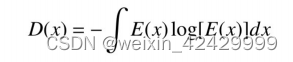
 其中，E（x）指的是连续的脑电信号的概率密度函数．

微分熵的代码实现

def compute_DE(signal):    #计算微分熵
    variance = np.var(signal, ddof=1)
    return math.log(2 * math.pi * math.e * variance) / 2

带通滤波

def butter_bandpass(lowcut, highcut, fs, order=5):  #带通滤波
    nyq = 0.5 * fs
    low = lowcut / nyq
    high = highcut / nyq
    b, a = butter(order, [low, high], btype='band')
    return b, a


def butter_bandpass_filter(data, lowcut, highcut, fs, order=5):
    b, a = butter_bandpass(lowcut, highcut, fs, order=order)
    y = lfilter(b, a, data)
    return y

什么要进行带通滤波呢？

因为对于原始数据，我们的目的是提取出四个频带（αβγθ）中的微分熵，所以我们要通过带通滤波从原始的信号中分离出这四个频带。（带通滤波器主要可以使用在需要保留的波的频率在一定的范围内，用于去除周围的噪声，可以起到良好的效果。）

加下来就是求出每次实验数据的微分熵了。

具体代码如下：

    for trial in range(40):  #对于其中40次试验,  这里是计算基线的DE特征
        temp_base_DE = np.empty([0])       #多一个基线DE
        temp_base_theta_DE = np.empty([0])   #相对于seed数据集在频带上少一个delta
        temp_base_alpha_DE = np.empty([0])
        temp_base_beta_DE = np.empty([0])
        temp_base_gamma_DE = np.empty([0])

        temp_de = np.empty([0, 120]) #将60S的数据进行一个切分，0.5s为一个点

        for channel in range(32):  #对于40次试验中的每次试验中的32个通道
            trial_signal = data[trial, channel, 384:]   #384之后的为试验数据
            base_signal = data[trial, channel, :384]  #384 为3*128=384前三秒为试验前基线
            # ****************compute base DE****************
            base_theta = butter_bandpass_filter(base_signal, 4, 8, frequency, order=3) #这里是对基线信号的处理
            base_alpha = butter_bandpass_filter(base_signal, 8, 14, frequency, order=3)
            base_beta = butter_bandpass_filter(base_signal, 14, 31, frequency, order=3)
            base_gamma = butter_bandpass_filter(base_signal, 31, 45, frequency, order=3)

            base_theta_DE = (compute_DE(base_theta[:64]) + compute_DE(base_theta[64:128]) + compute_DE(
                base_theta[128:192]) + compute_DE(base_theta[192:256]) + compute_DE(base_theta[256:320]) + compute_DE(
                base_theta[320:])) / 6  #首先用0.5s将基线分成6段，然后对这六段的DE特征进行一个平均
            base_alpha_DE = (compute_DE(base_alpha[:64]) + compute_DE(base_alpha[64:128]) + compute_DE(
                base_alpha[128:192]) + compute_DE(base_theta[192:256]) + compute_DE(base_theta[256:320]) + compute_DE(
                base_theta[320:])) / 6
            base_beta_DE = (compute_DE(base_beta[:64]) + compute_DE(base_beta[64:128]) + compute_DE(
                base_beta[128:192]) + compute_DE(base_theta[192:256]) + compute_DE(base_theta[256:320]) + compute_DE(
                base_theta[320:])) / 6
            base_gamma_DE = (compute_DE(base_gamma[:64]) + compute_DE(base_gamma[64:128]) + compute_DE(
                base_gamma[128:192]) + compute_DE(base_theta[192:256]) + compute_DE(base_theta[256:320]) + compute_DE(
                base_theta[320:])) / 6

            temp_base_theta_DE = np.append(temp_base_theta_DE, base_theta_DE)
            temp_base_gamma_DE = np.append(temp_base_gamma_DE, base_gamma_DE)
            temp_base_beta_DE = np.append(temp_base_beta_DE, base_beta_DE)
            temp_base_alpha_DE = np.append(temp_base_alpha_DE, base_alpha_DE)

            theta = butter_bandpass_filter(trial_signal, 4, 8, frequency, order=3)   #这是对实验数据的处理
            alpha = butter_bandpass_filter(trial_signal, 8, 14, frequency, order=3)
            beta = butter_bandpass_filter(trial_signal, 14, 31, frequency, order=3)
            gamma = butter_bandpass_filter(trial_signal, 31, 45, frequency, order=3)

            DE_theta = np.zeros(shape=[0], dtype=float)
            DE_alpha = np.zeros(shape=[0], dtype=float)
            DE_beta = np.zeros(shape=[0], dtype=float)
            DE_gamma = np.zeros(shape=[0], dtype=float)

            for index in range(120):
                DE_theta = np.append(DE_theta, compute_DE(theta[index * 64:(index + 1) * 64]))
                DE_alpha = np.append(DE_alpha, compute_DE(alpha[index * 64:(index + 1) * 64]))
                DE_beta = np.append(DE_beta, compute_DE(beta[index * 64:(index + 1) * 64]))
                DE_gamma = np.append(DE_gamma, compute_DE(gamma[index * 64:(index + 1) * 64]))
            temp_de = np.vstack([temp_de, DE_theta])
            temp_de = np.vstack([temp_de, DE_alpha])
            temp_de = np.vstack([temp_de, DE_beta])
            temp_de = np.vstack([temp_de, DE_gamma])
        temp_trial_de = temp_de.reshape(-1, 4, 120)
        decomposed_de = np.vstack([decomposed_de, temp_trial_de])

        #temp_base_DE = np.append(temp_base_DE, temp_base_theta_DE)
        temp_base_DE = np.append(temp_base_theta_DE, temp_base_alpha_DE)
        temp_base_DE = np.append(temp_base_DE, temp_base_beta_DE)
        temp_base_DE = np.append(temp_base_DE, temp_base_gamma_DE)
        base_DE = np.vstack([base_DE, temp_base_DE])

最后我们得到的数据形式为【4800，128】

接下来我们要把数据规模改变为对应频带，电极二维映射的形式，也就是【4800，4，9，9】

也就是这种形式：

 当我们把数据处理工作完成后，我们就可以把数据集划分为训练集以及测试集，（一般采用K折交叉验证。）然后把分好的数据放到网络里进行训练与测试 。

class ConvLSTM(nn.Module):
    def __init__(self, embedding_size, batch_size, num_classes, hidden_size=8, num_directions=1, num_layers=1):
        super(ConvLSTM, self).__init__()
        self.conv1 = nn.Conv2d(4, 24, 5)

        self.conv2 = nn.Conv2d(24, 128, 2)
        self.fc1 = nn.Linear(128 * 2 * 2, 96)
        self.fc2 = nn.Linear(96, embedding_size)
        self.lstm = nn.LSTM(embedding_size, hidden_size, num_layers, batch_first=True)
        self.hidden = None
        self.init_hidden(batch_size, hidden_size, num_directions, num_layers)
        self.fc3 = nn.Linear(hidden_size, num_classes)

 最后的结果为：