数据驱动分析实践三 Customer Lifetime Value

数据驱动分析三

Customer Lifetime Value

    上一篇我们探讨了如何进行客户分段，并介绍了RFM方法。本篇我们进入了本系列最重要的主题，如何估算CLV(Customer Lifetime Value)。关于CLV的基本概念和理论，读者可参见本人的另外系列文章用户存续期价值评估

    事实上，我们经常在客户上投入以获得收入及利润，例如获客成本、线下广告、宣传活动和折扣等。这些活动自然而然地会产生价值非常高的客户，当然也会存在降低利润的客户。我们需要辨别出这些不同客户的行为特点，进行客户分段并采取相应的行为。

    计算CLV并不是一个很难的事，一般我们可以选定一个时间窗口，按照下面的公式计算。
CLV = Total Gross Value - Total cost

    这个公式只能告诉我们历史信息，当发现一个客户的价值为负时，可能已经太晚了。在这种情况下，我们尝试使用机器学习来预测未来的CLV.

预测CLV

    我们将采用如下步骤：

• 为CLV的计算定义时间窗口
• 特征工程
• 构建和训练机器学习模型
• 运行模型
• 检验模型有效性

    如何定义时间窗口依赖于所在行业、商业模式、战略等因素。对某些行业来说，一年已经是较长的时间窗口了，但对于另外一些行业就属于比较短的窗口。我们在这个演示例子中使用6个月的时间窗口。

    在上一篇文章中，我们已经为每一个客户计算过了RFM评分，这个分数是一个良好的特征。本文中，我们将会拆分我们的数据集，计算三个月的RFM且使用它来计算下六个月的值。

#import libraries
from __future__ import division
from datetime import datetime, timedelta,date
import pandas as pd
%matplotlib inline
from sklearn.metrics import classification_report,confusion_matrix
import matplotlib.pyplot as plt
import numpy as np
import seaborn as sns

from sklearn.cluster import KMeans
import chart_studio.plotly as py
import plotly.offline as pyoff
import plotly.graph_objs as go

#import plotly.plotly as py
#import plotly.offline as pyoff
#import plotly.graph_objs as go

import xgboost as xgb
from sklearn.model_selection import KFold, cross_val_score, train_test_split

import xgboost as xgb

#initate plotly
pyoff.init_notebook_mode()

#read data from csv and redo the data work we done before
tx_data = pd.read_excel('Online Retail.xlsx')
tx_data['InvoiceDate'] = pd.to_datetime(tx_data['InvoiceDate'])
tx_uk = tx_data.query("Country=='United Kingdom'").reset_index(drop=True)

#create 3m and 6m dataframes
tx_3m = tx_uk[(tx_uk.InvoiceDate < datetime(2011,6,1)) & (tx_uk.InvoiceDate >= datetime(2011,3,1))].reset_index(drop=True)
tx_6m = tx_uk[(tx_uk.InvoiceDate >= datetime(2011,6,1)) & (tx_uk.InvoiceDate < datetime(2011,12,1))].reset_index(drop=True)

#create tx_user for assigning clustering
tx_user = pd.DataFrame(tx_3m['CustomerID'].unique())
tx_user.columns = ['CustomerID']

#order cluster method
def order_cluster(cluster_field_name, target_field_name,df,ascending):
    new_cluster_field_name = 'new_' + cluster_field_name
    df_new = df.groupby(cluster_field_name)[target_field_name].mean().reset_index()
    df_new = df_new.sort_values(by=target_field_name,ascending=ascending).reset_index(drop=True)
    df_new['index'] = df_new.index
    df_final = pd.merge(df,df_new[[cluster_field_name,'index']], on=cluster_field_name)
    df_final = df_final.drop([cluster_field_name],axis=1)
    df_final = df_final.rename(columns={"index":cluster_field_name})
    return df_final


#calculate recency score
tx_max_purchase = tx_3m.groupby('CustomerID').InvoiceDate.max().reset_index()
tx_max_purchase.columns = ['CustomerID','MaxPurchaseDate']
tx_max_purchase['Recency'] = (tx_max_purchase['MaxPurchaseDate'].max() - tx_max_purchase['MaxPurchaseDate']).dt.days
tx_user = pd.merge(tx_user, tx_max_purchase[['CustomerID','Recency']], on='CustomerID')

kmeans = KMeans(n_clusters=4)
kmeans.fit(tx_user[['Recency']])
tx_user['RecencyCluster'] = kmeans.predict(tx_user[['Recency']])

tx_user = order_cluster('RecencyCluster', 'Recency',tx_user,False)

#calcuate frequency score
tx_frequency = tx_3m.groupby('CustomerID').InvoiceDate.count().reset_index()
tx_frequency.columns = ['CustomerID','Frequency']
tx_user = pd.merge(tx_user, tx_frequency, on='CustomerID')

kmeans = KMeans(n_clusters=4)
kmeans.fit(tx_user[['Frequency']])
tx_user['FrequencyCluster'] = kmeans.predict(tx_user[['Frequency']])

tx_user = order_cluster('FrequencyCluster', 'Frequency',tx_user,True)

#calcuate revenue score
tx_3m['Revenue'] = tx_3m['UnitPrice'] * tx_3m['Quantity']
tx_revenue = tx_3m.groupby('CustomerID').Revenue.sum().reset_index()
tx_user = pd.merge(tx_user, tx_revenue, on='CustomerID')

kmeans = KMeans(n_clusters=4)
kmeans.fit(tx_user[['Revenue']])
tx_user['RevenueCluster'] = kmeans.predict(tx_user[['Revenue']])
tx_user = order_cluster('RevenueCluster', 'Revenue',tx_user,True)


#overall scoring
tx_user['OverallScore'] = tx_user['RecencyCluster'] + tx_user['FrequencyCluster'] + tx_user['RevenueCluster']
tx_user['Segment'] = 'Low-Value'
tx_user.loc[tx_user['OverallScore']>2,'Segment'] = 'Mid-Value' 
tx_user.loc[tx_user['OverallScore']>4,'Segment'] = 'High-Value' 

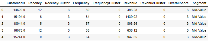
这里就不再重复RFM评分的细节，因为已经在上一篇文章中详细介绍过。

tx_user.head()

特征集已经准备好了，下一步我们来计算6个月的每个客户的LTV，结果会被用来训练我们的模型。

本例数据集中并没有定义成本(cost)，所以收入(Revenue)就会被当成LTV。

#calculate revenue and create a new dataframe for it
tx_6m['Revenue'] = tx_6m['UnitPrice'] * tx_6m['Quantity']
tx_user_6m = tx_6m.groupby('CustomerID')['Revenue'].sum().reset_index()
tx_user_6m.columns = ['CustomerID','m6_Revenue']


#plot LTV histogram
plot_data = [
    go.Histogram(
        x=tx_user_6m.query('m6_Revenue < 10000')['m6_Revenue']
    )
]

plot_layout = go.Layout(
        title='6m Revenue'
    )
fig = go.Figure(data=plot_data, layout=plot_layout)
pyoff.iplot(fig)

    上面计算了LTV并画出了其直方图。直方图中可以看出我们有一些客户的LTV为负；且存在一些异常值，过滤掉异常值会使机器学习模型更加健壮。

    下一步，我们将会合并3个月和6个月的数据，观察一下LTC和特征集之间的相关性。

tx_merge = pd.merge(tx_user, tx_user_6m, on='CustomerID', how='left')
tx_merge = tx_merge.fillna(0)

tx_graph = tx_merge.query("m6_Revenue < 30000")

plot_data = [
    go.Scatter(
        x=tx_graph.query("Segment == 'Low-Value'")['OverallScore'],
        y=tx_graph.query("Segment == 'Low-Value'")['m6_Revenue'],
        mode='markers',
        name='Low',
        marker= dict(size= 7,
            line= dict(width=1),
            color= 'blue',
            opacity= 0.8
           )
    ),
        go.Scatter(
        x=tx_graph.query("Segment == 'Mid-Value'")['OverallScore'],
        y=tx_graph.query("Segment == 'Mid-Value'")['m6_Revenue'],
        mode='markers',
        name='Mid',
        marker= dict(size= 9,
            line= dict(width=1),
            color= 'green',
            opacity= 0.5
           )
    ),
        go.Scatter(
        x=tx_graph.query("Segment == 'High-Value'")['OverallScore'],
        y=tx_graph.query("Segment == 'High-Value'")['m6_Revenue'],
        mode='markers',
        name='High',
        marker= dict(size= 11,
            line= dict(width=1),
            color= 'red',
            opacity= 0.9
           )
    ),
]

plot_layout = go.Layout(
        yaxis= {'title': "6m LTV"},
        xaxis= {'title': "RFM Score"},
        title='LTV'
    )
fig = go.Figure(data=plot_data, layout=plot_layout)
pyoff.iplot(fig)

    从图中我们可以看到LTV和RFM Scores还是存在正向关系的。

    在构建机器学习模型之前，我们需要确定采用何种机器学习算法。LTV本身是一个回归问题，机器学习模型可以预测LTV值。但是我们需要对LTV进行分段。因为分段使之更具备可操作性和更方便与人沟通。可使用Kmeans聚类算法，我们能够确定已经存在的LTV组，且在其上进行分段。

    考虑到这个分析的商业部分，我们需要基于所预测的客户的LTV值，区别对待每个客户。在这个例子中，我们将使用聚类算法并进行三分段。实际情况下，分段的个数取决于业务的动态变化和目标。

• Low LTV
• Mid LTV
• High LTV

#remove outliers
tx_merge = tx_merge[tx_merge['m6_Revenue']<tx_merge['m6_Revenue'].quantile(0.99)]


#creating 3 clusters
kmeans = KMeans(n_clusters=3)
kmeans.fit(tx_merge[['m6_Revenue']])
tx_merge['LTVCluster'] = kmeans.predict(tx_merge[['m6_Revenue']])

#order cluster number based on LTV
tx_merge = order_cluster('LTVCluster', 'm6_Revenue',tx_merge,True)

#creatinga new cluster dataframe
tx_cluster = tx_merge.copy()

#see details of the clusters
tx_cluster.groupby('LTVCluster')['m6_Revenue'].describe()

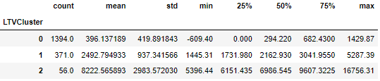
    LTVCluster为2的是最好的，它的平均LTV为8k;0 是最差的，平均LTV只有396.

    在训练机器学习模型之前，还需要做一些事情：

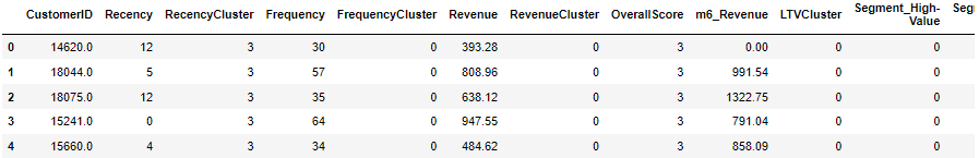
• 特征工程，需要将一些分类变量转化为数值变量。
• 检查各个特征和LTV的相关性。
• 划分训练集和测试集。

#convert categorical columns to numerical
tx_class = pd.get_dummies(tx_cluster)

#calculate and show correlations
corr_matrix = tx_class.corr()
corr_matrix['LTVCluster'].sort_values(ascending=False)

#create X and y, X will be feature set and y is the label - LTV
X = tx_class.drop(['LTVCluster','m6_Revenue'],axis=1)
y = tx_class['LTVCluster']

#split training and test sets
X_train, X_test, y_train, y_test = train_test_split(X, y, test_size=0.05, random_state=56)

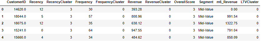
tx_cluster.head()

tx_class.head()

corr_matrix['LTVCluster'].sort_values(ascending=False)

LTVCluster 1.000000
m6_Revenue 0.845933
Revenue 0.600491
RevenueCluster 0.463930
OverallScore 0.373231
FrequencyCluster 0.366366
Frequency 0.359601
Segment_High-Value 0.353218
RecencyCluster 0.236899
Segment_Mid-Value 0.166854
CustomerID -0.028401
Recency -0.237249
Segment_Low-Value -0.266008
Name: LTVCluster, dtype: float64

    从相关矩阵中看到收入、频率、RFM Score对这个预测模型会比较有价值。

构建xgboost预测模型

#XGBoost Multiclassification Model
ltv_xgb_model = xgb.XGBClassifier(max_depth=5, learning_rate=0.1,objective= 'multi:softprob',n_jobs=-1).fit(X_train, y_train)

print('Accuracy of XGB classifier on training set: {:.2f}'
       .format(ltv_xgb_model.score(X_train, y_train)))
print('Accuracy of XGB classifier on test set: {:.2f}'
       .format(ltv_xgb_model.score(X_test[X_train.columns], y_test)))

y_pred = ltv_xgb_model.predict(X_test)
print(classification_report(y_test, y_pred))

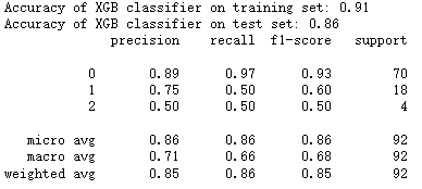
正确率在测试集上显示为86%，这个结果如何呢？
    我们需要对模型质量进行检查。LTVCluster0的数量占总数的76.5%，如果我们把所有客户都划分到Cluster0，我们也可以获得76.5&的准确率。 86% VS 76.5%说明这个模型是有用的，但可能需要进一步调整和优化。请看下面的分类报告:

print(classification_report(y_test,y_pred))

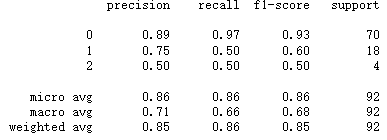
    对于Cluster0(low LTV)来说，其准确率(precison)和召回率(recall)是不错的；但是对于Mid LTV和High LTV就不是很好了，可以考虑从以下几个方面入手来优化模型：

• 增加更多的特征并进行更深一步的特征工程
• 尝试其他模型
• 对xgboost模型进行参数优化调整
• 增加更多的数据

    好!我们已经拥有了一个预测客户LTV分段的机器学习模型。我们可以根据模型的结果采取相应的措施。显然，我们不想失去具有高LTV的客户。所以再下一篇文章我们将讨论留存分析。

未完待续，…