


ESDA in PySAL (1) 利用 A-DBSCAN 聚类点并探索边界模糊性
在本例中,我们将以柏林的 AirBnb 房源样本为例,说明如何使用 A-DBSCAN (Arribas-Bel et al., 2019)。A-DBSCAN 可以让我们做两件事:
- 识别高密度 AirBnb 房源集群并划定其边界
- 探索这些边界的稳定性
%matplotlib inline

import pandas
import geopandas
import numpy as np
import contextily as cx
import matplotlib.pyplot as plt
from shapely.geometry import Polygon
from libpysal.cg.alpha_shapes import alpha_shape_auto

import sys
sys.path.append("../")
try:
    from esda.adbscan import ADBSCAN, get_cluster_boundary, remap_lbls
# This below can be removed once A-DBSCAN is merged into `esda`
except:
    print("Import from local folder...")
    import sys
    sys.path.append("../esda")
    from adbscan import ADBSCAN, get_cluster_boundary, remap_lbls
数据
我们将使用 Inside Airbnb 中的柏林提取数据。这与 Scipy 2018 tutorial on Geospatial data analysis with Python中使用的数据集相同。
tab = pandas.read_csv("data/berlin-listings.csv")
tab.head(2)
| Unnamed: 0 | id | listing_url | scrape_id | last_scraped | name | summary | space | description | experiences_offered | ... | review_scores_value | requires_license | license | jurisdiction_names | instant_bookable | cancellation_policy | require_guest_profile_picture | require_guest_phone_verification | calculated_host_listings_count | reviews_per_month | |
|---|---|---|---|---|---|---|---|---|---|---|---|---|---|---|---|---|---|---|---|---|---|
| 0 | 0 | 17260587 | https://www.airbnb.com/rooms/17260587 | 20170507222235 | 2017-05-08 | Kunterbuntes Zimmer mit eigenem Bad für jedermann | Meine Unterkunft ist gut für paare, alleinreis... | NaN | Meine Unterkunft ist gut für paare, alleinreis... | none | ... | 10.0 | f | NaN | NaN | t | flexible | f | f | 3 | 2.00 |
| 1 | 1 | 17227881 | https://www.airbnb.com/rooms/17227881 | 20170507222235 | 2017-05-08 | Modernes Zimmer in Berlin Pankow | Es ist ein schönes gepflegtes und modernes Zim... | Das Haus befindet sich direkt vor eine Tram Ha... | Es ist ein schönes gepflegtes und modernes Zim... | none | ... | 10.0 | f | NaN | NaN | t | flexible | f | f | 1 | 1.29 |
2 rows × 96 columns
原始数据集包括 20,000 多个观测值:
tab.shape
(20053, 96)
为了让图解在任何硬件上运行得更快一些,让我们随机抽取 10%的样本,即随机抽取 2,000 个属性:
tab = tab.sample(n=2000, random_state=1234)
为方便起见,我们将其转换为 “GeoDataFrame”,其中的几何图形是根据原始表格中的长/纬度列建立的:
db_ll = geopandas.GeoDataFrame(tab,
                               geometry=geopandas.points_from_xy(tab.longitude, tab.latitude),
                               crs={'init': 'epsg:4326'}
                              )
/home/serge/anaconda3/envs/analytical/lib/python3.7/site-packages/pyproj/crs/crs.py:53: FutureWarning: '+init=<authority>:<code>' syntax is deprecated. '<authority>:<code>' is the preferred initialization method. When making the change, be mindful of axis order changes: https://pyproj4.github.io/pyproj/stable/gotchas.html#axis-order-changes-in-proj-6
  return _prepare_from_string(" ".join(pjargs))
因为我们要运行一个依赖于距离的算法,所以我们需要能够在投影平面上计算这些距离。我们使用为德国设计的ETRS89投影来代替原始的长/纬度坐标,并以米为单位:
db = db_ll.to_crs(epsg=5243)
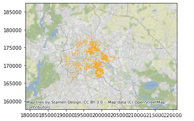
*现在我们可以将数据集可视化了:
ax = db.plot(markersize=0.1, color='orange')
cx.add_basemap(ax, crs=db.crs.to_string());
在开始之前,我们还将把投影坐标分成不同的列:
db["X"] = db.geometry.x
db["Y"] = db.geometry.y
识别 AirBnb 的聚类
A-DBSCAN 与最初的 DBSCAN 算法类似,运行前需要两个参数:
- eps`:从每个地点寻找邻居的最大距离
- min_samples`:一个点被视为聚类的一部分所需的最小相邻点数
在本例中,我们将选取总体样本量的 1% 作为 min_samples 参数:
db.shape[0] * 0.01
20.0
我们将使用 500 米的最大弧度作为 eps 参数。这隐含着我们正在寻找的是每平方千米
K
m
2
Km^2
Km2 至少约 25 个属性的密度(
d
e
n
s
=
20
p
i
×
0.
5
2
dens = \frac{20}{pi\, \times\, 0.5^2}
dens=pi×0.5220)。
知道要使用的参数后,我们就可以继续运行 A-DBSCAN:
%%time
# Get clusters
adbs = ADBSCAN(500, 20, pct_exact=0.5, reps=10, keep_solus=True)
np.random.seed(1234)
adbs.fit(db)
CPU times: user 755 ms, sys: 3.36 ms, total: 758 ms
Wall time: 752 ms


ADBSCAN(eps=500, keep_solus=True, min_samples=20, pct_exact=0.5, reps=10)
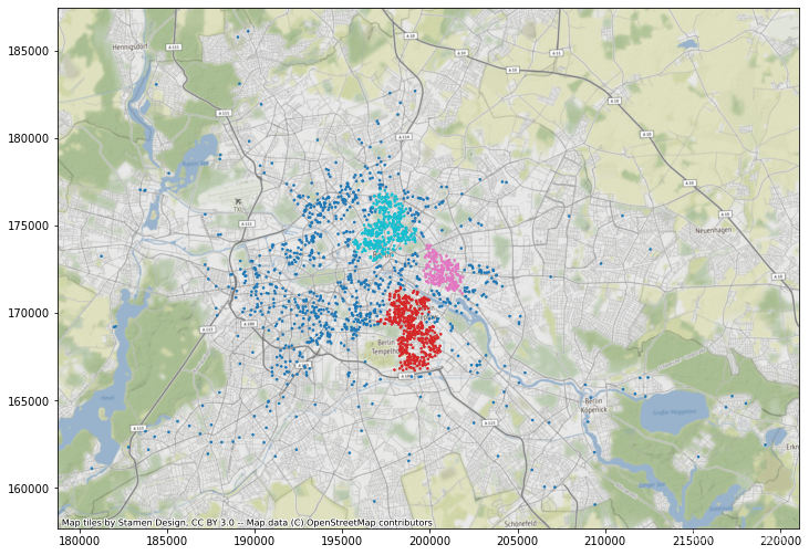
一旦 "fit() "成功,我们就能以类似于 "scikit-learn "的方式提取标签,然后绘制地图:
ax = db.assign(lbls=adbs.votes["lbls"])\
       .plot(column="lbls",
             categorical=True,
             markersize=2.5,
             figsize=(12, 12)
            )
cx.add_basemap(ax, crs=db.crs.to_string());
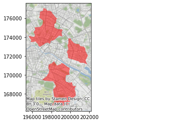
这只会显示根据标签分配的每个属性的颜色。除此以外,我们还可以创建多边形,表示特定聚类中所有点的紧密边界。为此,我们通过辅助函数 get_cluster_boundary 使用
α
\alpha
α-shapes 算法:
%time polys = get_cluster_boundary(adbs.votes["lbls"], db, crs=db.crs)
CPU times: user 1.76 s, sys: 15.2 ms, total: 1.78 s
Wall time: 1.77 s
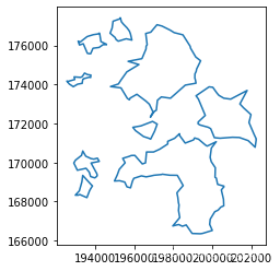
这些多边形也可以像其他 "地理系列 "对象一样绘制:
ax = polys.plot(alpha=0.5, color="red")
cx.add_basemap(ax, crs=polys.crs.to_string());
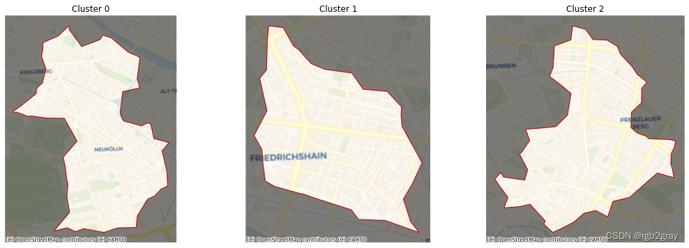
为了好玩,我们还可以创建更多的放大视图,将每个星团外的区域调暗:
f, axs = plt.subplots(1, 3, figsize=(18, 6))
for i, ax in enumerate(axs):
    # Plot the boundary of the cluster found
    ax = polys[[i]].plot(ax=ax,
                         edgecolor="red",
                         facecolor="none"
                        )
    # Add basemap
    cx.add_basemap(ax,
                   crs=polys.crs.to_string(),
                   url=cx.providers.CartoDB.Voyager,
                   zoom=13
                  )
    # Extra to dim non-cluster areas
    (minX, maxX), (minY, maxY) = ax.get_xlim(), ax.get_ylim()
    bb = Polygon([(minX, minY),
                  (maxX, minY),
                  (maxX, maxY),
                  (minX, maxY),
                  (minX, minY)
                 ])
    geopandas.GeoSeries([bb.difference(polys[i])],
                        crs=polys.crs
                       ).plot(ax=ax,
                              color='k',
                              alpha=0.5
                             )
    ax.set_axis_off()
    ax.set_title(f"Cluster {polys[[i]].index[0]}")
plt.show()
/home/serge/anaconda3/envs/analytical/lib/python3.7/site-packages/ipykernel_launcher.py:12: FutureWarning: The "url" option is deprecated. Please use the "source" argument instead.
  if sys.path[0] == '':
/home/serge/anaconda3/envs/analytical/lib/python3.7/site-packages/ipykernel_launcher.py:12: FutureWarning: The "url" option is deprecated. Please use the "source" argument instead.
  if sys.path[0] == '':
/home/serge/anaconda3/envs/analytical/lib/python3.7/site-packages/ipykernel_launcher.py:12: FutureWarning: The "url" option is deprecated. Please use the "source" argument instead.
  if sys.path[0] == '':
探索边界的模糊性
A-DBSCAN 的主要优点之一是,由于它依赖于生成多个候选解的集合方法,因此我们可以探索边界在多大程度上是稳定、清晰或模糊的。为此,我们需要从 ADBSCAN 对象中提取每个候选解,并将其转化为边界线(这可能需要运行一段时间):
%%time
solus_rl = remap_lbls(adbs.solus, db, n_jobs=-1)
lines = []
for rep in solus_rl:
    line = get_cluster_boundary(solus_rl[rep],
                                db,
                                crs=db.crs,
                                n_jobs=-1
                               )
    line = line.boundary
    line = line.reset_index()\
               .rename(columns={0: "geometry",
                                "index": "cluster_id"}
                      )\
               .assign(rep=rep)
    lines.append(line)
lines = pandas.concat(lines)
lines = geopandas.GeoDataFrame(lines, crs=db.crs)
CPU times: user 665 ms, sys: 1.45 s, total: 2.12 s
Wall time: 4.83 s
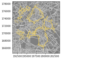
下面是模拟得出的所有解决方案的初探:
ax = lines.plot(color="#FFDB58",
                linewidth=0.5
               )
cx.add_basemap(ax,
               alpha=0.5,
               url=cx.providers.Stamen.TonerHybrid,
               crs=lines.crs.to_string()
              )
/home/serge/anaconda3/envs/analytical/lib/python3.7/site-packages/ipykernel_launcher.py:7: FutureWarning: The "url" option is deprecated. Please use the "source" argument instead.
  import sys
将每个候选边界存储和标记到一个表中,我们就可以进行多次查询。例如,以下是第一次复制产生的所有解决方案:
lines.query("rep == 'rep-00'").plot()
<matplotlib.axes._subplots.AxesSubplot at 0x7fc0003522d0>
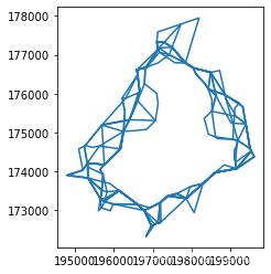
这就是第 2 组标签的所有候选方案:
lines.query("cluster_id == '2'").plot()
<matplotlib.axes._subplots.AxesSubplot at 0x7fc000452e90>
最后,我们还可以将这一想法应用到交互式环境中,通过构建小工具来刷新复制:
from ipywidgets import interact, IntSlider
def plot_rep(rep):
    f, ax = plt.subplots(1, figsize=(9, 9))
    ax.set_facecolor("k")
    # Background points
    db[["X", "Y"]].plot.scatter("X", "Y", ax=ax, color="0.25", s=0.5)
    # Boundaries
    cs = lines.query(f"rep == 'rep-{str(rep).zfill(2)}'")
    cs.plot(ax=ax, color="red")
    # Cluster IDs
    for s, row in cs.iterrows():
        ax.text(row.geometry.centroid.x,
                row.geometry.centroid.y,
                s,
                size=20,
                c="w"
               )
    return None
reps = range(len(lines["rep"].unique()))
slider = IntSlider(min=min(reps), max=max(reps), step=1)
interact(plot_rep, rep=slider);
interactive(children=(IntSlider(value=0, description='rep', max=9), Output()), _dom_classes=('widget-interact'…
或者为给定的集群 ID 调出所有解决方案:
def plot_cluster(cluster_id):
    f, ax = plt.subplots(1, figsize=(9, 9))
    ax.set_facecolor("k")
    # Background points
    db[["X", "Y"]].plot.scatter("X",
                                "Y",
                                ax=ax,
                                color="0.25",
                                s=0.5,
                                alpha=0.5
                               )
    # Boundaries
    lines.query(f"cluster_id == '{cluster_id}'").plot(ax=ax,
                                                      linewidth=1,
                                                      alpha=0.5
                                                     )
    return None
interact(plot_cluster, cluster_id=lines["cluster_id"].unique());


 5266
5266

 被折叠的 条评论
为什么被折叠?
被折叠的 条评论
为什么被折叠?
 到【灌水乐园】发言


