第10章. 预测和不确定性分析

A good forecaster is not smarter than everyone else, he merely has his ignorance better organized.

——Anonymous

There are known knowns. These are things we know that we know. There are known unknowns. That is to say, there are things that we now know we don’t know. But there are also unknown unknowns. These are things we do not know we don’t know.

——Donald Rumsfeld

10.1 INTRODUCTION 

For most applied groundwater modeling problems, the model’s purpose is addressed by making a forecast of the response of the system to future conditions, or (less frequently) a backcast or hindcast to past conditions (Fig. 10.1). We use the term forecast over prediction to reflect the fact that all estimates of future conditions have uncertainty; the term forecast more accurately represents that inherent uncertainty. There is also widespread understanding of forecast probability (e.g., “70% chance of rain”) among scientists and the general public, whereas “prediction” connotes more certainty. A forecast is considered acceptable when it adequately represents all that is known at the time of the forecast, even though what was forecast may not come to pass owing to factors unknown when the forecast was made.

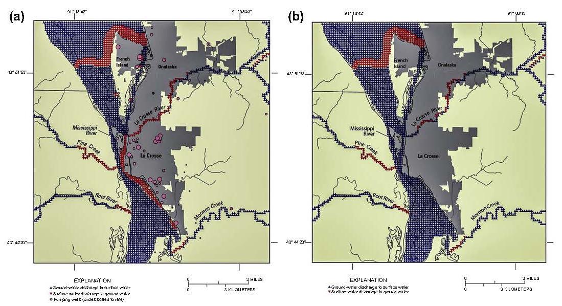
Figure 10.1 A simple example of hindcasting groundwateresurface water interaction in a humid temperate climate (Wisconsin, USA). A model calibrated to current pumping conditions (a) is re-run to simulate groundwateresurface water interaction before pumping (b). Red symbols identify areas of induced flow from surface water in response to pumping, a dam, and high hydraulic conductivity fluvial sediments in the river valleys. Blue symbols represent areas of groundwater discharge to surface water. Comparison of (a) and (b) shows the expansion of losing stream conditions caused by pumping. The effect of the dam is evident during both time periods (horizontal red band near top of figures) (modified from Hunt et al, 2003).

In a forecasting simulation, future changes in the groundwater system are typically simulated using a calibrated model, which is called the base model. The base model is founded on a conceptual model supported by field data, and is calibrated by history matching to provide the subjective (weighted) best fit to calibration targets and soft knowledge. It is not considered a true or complete representation of actual groundwater conditions. Instead, it is recognized to contain parameter error from both observation measurement error and parameter simplification errors such that the model is unable to capture all system detail (Chapter 9). Not all forecasts require calibrated models, however. Uncalibrated interpretive models (Section 1.3) can also be used to explore how changes in properties or assumptions influence outcomes of interest, or used to explore best- or worst-case scenarios (e.g., Doherty and Simmons, 2013). However, in this chapter, we focus on forecasting using a base model.

Groundwater modeling forecasts are often used to plan future actions because they help characterize the likelihood that something “bad” might happen (Freeze et al, 1990; Tartakovsky, 2013), such as an ecologically sensitive stream going dry or a water withdrawal exceeding what is sustainable. The role of forecasting in this context is to assess likelihood of an event, which is a concept very different from predicting what will happen in the future (Doherty, 2011). Modeling expresses our lack of knowledge because even a perfectly calibrated model cannot guarantee that a forecast is accurate. Yet with a reasonable model, formal cost-benefit or risk-assessment analyses can be performed by including a quantification of uncertainty (e.g., Tartakovsky, 2013). It is critical that the model be reasonable. As noted by Silver (2012): It is forecasting’s original sin to put politics, personal glory, or economic benefit before the truth of the forecast. Sometimes it is done with good intentions, but it always makes the forecast worse.

Here, truth means that the forecast is an unbiased and fair depiction of what is expected to occur. It is the obligation of the modeler to provide the best forecast possible, report uncertainty bounds around the forecast, and communicate those limits in an understandable way to other modelers, clients, managers, and regulators. Indeed, it has been argued that model forecasts submitted without uncertainty estimates should be rejected out of hand (Beven and Young, 2013).

Although the importance of characterizing uncertainty has been recognized for a long time (e.g., Knight, 1921), there is still “uncertainty about uncertainty estimation in environmental modeling” (Beven, 2005). Many of the tools used to quantify uncertainty in groundwater modeling were developed in other branches of science. For example, real-time forecasting of flood stages, projecting changes in atmospheric CO2, making weather forecasts, and anticipating changes in stock market value, all commonly include uncertainty analyses. A brief historical overview in Box 10.1 gives a short history of uncertainty techniques in groundwater modeling. Such a historical snapshot is necessarily incomplete, however, as the topic is large and evolving, and there is no agreed upon fundamental set of approaches applicable to the wide range of modeling objectives being addressed. Finally, it should be noted that throughout this chapter “uncertainty” and “error” are used interchangeably for convenience, though there are advantages to considering them conceptually separate (e.g., White et al, 2014).

---

Box 10.1 Historical Overview of Un