GMS User Manual (v10.3)_gms:user-CSDN博客

本文链接：https://blog.csdn.net/weixin_44259522/article/details/135536759

Groundwater Modeling System

Learning GMS

What Is GMS

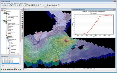
SUB package vertical displacement plot.

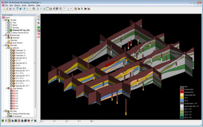
Solid cross sections and boreholes.

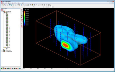
Isosurface on a 3D grid and borehole sample data.

The Groundwater Modeling System (GMS) is a comprehensive graphical user environment for performing groundwater simulations. The entire GMS system consists of a graphical user interface (the GMS program) and a number of analysis codes (MODFLOW, MT3DMS, etc.). The GMS interface is developed by Aquaveo, LLC in Provo, Utah.

GMS was designed as a comprehensive modeling environment. Several types of models are supported and facilities are provided to share information between different models and data types. Tools are provided for site characterization, model conceptualization, mesh and grid generation, geostatistics, and post-processing.

Modules

The interface for GMS is divided into twelve modules. A module is provided for each of the basic data types supported by GMS. As you switch from one module to another module, the Dynamic Tool Palette and the Menus change. This allows you to focus only on the tools and commands related to the data type you wish to use in the modeling process. The following modules are supported in GMS:

Icon	Module
	TIN Module
	Borehole Module
	Solid Module
	2D Mesh Module
	2D Grid Module
	2D Scatter Point Module
	3D Mesh Module
	3D Grid Module
	3D Scatter Point Module
	Map Module
	GIS Module
	UGrid Module

Numerical Models

Numerical models are programs that are separate from GMS that are used to run an analysis on a simulation. The simulation can be built in GMS, and then run through the numerical model program. GMS can then read in and display the results of the analysis.

The following numerical models are currently supported in GMS:

Model Name	GMS Module
MODFLOW MODPATH MT3DMS PEST PHT3D RT3D SEAWAT SEAM3D	3D Grid
MODAEM UTEXAS	Map Module
SEEP2D	2D Mesh
FEMWATER	3D Mesh
T-PROGS	Boreholes

Source code for most models is available upon request. Contact technical support to request source code.

What's New in GMS 10.3

The following is a list of the more significant changes that will be introduced in GMS 10.3.

MODFLOW
1. Support for preserving DISU data created outside of GMS

1. Map -> CLN
2. Update to PEST 14.0

1. Update to MODFLOW-NWT 1.1.2
2. Support for SYTP parameter type for HUF package

1. Zone flow for MODFLOW-USG ZoneBudget (GMS Feature Request)
2. Mapping SFR2 to multiple surface layers (GMS Feature Request)

MT3D-USGS
1. New model added to GMS

mod-PATH3DU
1. Support for version 1.1.0 including new Waterloo method and modified grid specification file

1. Support for DefaultIFACE
2. Model Checker added to find obvious model setup errors

1. Model Wrapper and automatic reading of the solution
2. Export options to save shapefiles of pathlines, pathline points, and polygon capture zones

1. Option to create starting locations from UGrid points or cell centers
2. Interface taken out of beta

UGrids
1. Display Options per UGrid
2. Split a UGrid layer (GMS Feature Request)

New Tutorials
1. mod-PATH3DU Transient tutorial
2. MT3D-USGS Tutorial

1. Shapefile to CLN
2. Recharge

Miscellaneous
1. * Higher resolution bitmaps for use on higher resolution displays
2. Get Data Tool for downloading online data for a polygonal area

1. Improved 2D mesh generation
2. Change to dialog that asks about saving changes on File|New

1. Export 3D Grid layer contours to a shapefile.
2. New Empty UGrid 2D command for creating UGrids that points will be added to (like a TIN or 2D Scatter Set)

1. Notes (GMS Feature Request)
2. Time format options (GMS Feature Request)

1. Export multiple particle sets to shapefiles (GMS Feature Request)
2. Include starting cell in pathline report for MODPATH, MP3DU (GMS Feature Request)

1. TOB enhancements: iConcINTP set to 1 by default, add the well id to the comment lines in the header of the TOBS input file (GMS Feature Request)
2. Reuse PEST Jacobian (GMS Feature Request)

1. Option to export only active grid cells to shapefile (GMS Feature Request)
2. Pathline arrows (time markers) to shapefile (GMS Feature Request)

* In progress

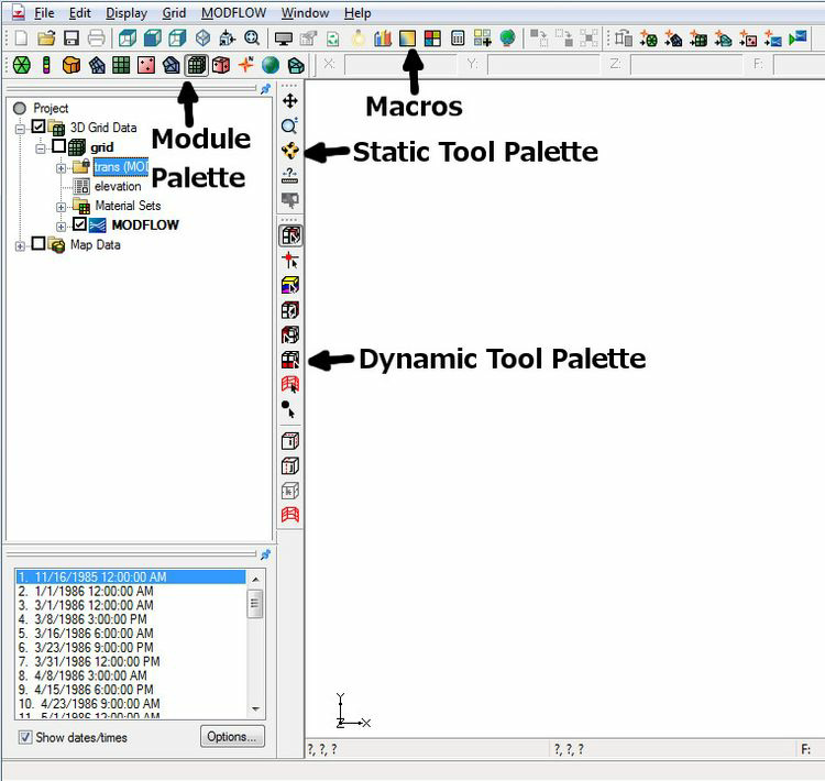
The GMS Window

The GMS window is divided into seven main sections:

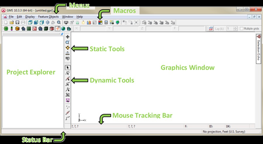The GMS window with different parts labeled.

Menus

The File, Edit, Display, Window and Help menus are always available. Other menus change based on the module or numerical model in use.

Toolbars

For a full description of all the toolbars, see Toolbars.

Shortcut Toolbars

The shortcut toolbars are shortcuts (sometimes referred to as "macros") to often used menu commands.

Module toolbar

The module toolbar let's switching between modules.

XYZF Bar

These fields are used to edit the coordinates and scalar data set values of selected items (vertices, nodes, scatter points, etc.).

Project Explorer

The Project Explorer contains a hierarchical representation of the data associated with a modeling project.

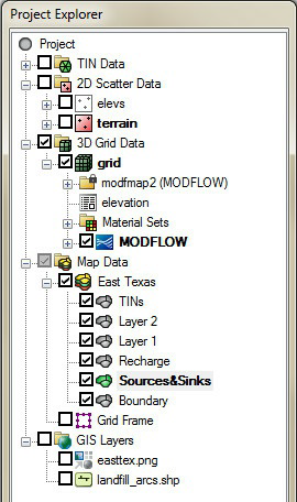Example of the Project Explorer

Static and Dynamic Tools

The static and dynamic tools change the behavior of the mouse in the Graphics Window. The static tools are the same for every module and the dynamic tools change depending on the module. The dynamic tools typically are for creation or selection of objects.

Graphics Window

The Graphics Window is where data is rendered and data is manipulated using tools.

Mouse Tracking Bar

This shows the real world coordinates of the mouse in the Graphics Window. If the mouse is over a cell, triangle or element, the F value is the dataset scalar value and the ID is the object's number. For 3D Grids, the IJK of the cell is also shown. The progress bar is also found here.

Selection Echo

This allows quickly viewing the properties of a selected object, point, node, cell, or element.

Status Bar

The Status Bar is used to display messages and information about selected items. It also shows the display projection.

Time Steps Window

The Time Steps window is available only when a dataset containing a time series is active in the Project Explorer. The window allows selecting individual time steps for display in the Graphics Window. The window is usually located beneath the Project Explorer, but is can be resized and/or unpinned to be it's own window.

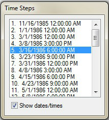Example of the Time Steps window.

Toolbars

There are several toolbars that can be displayed in the GMS interface. Below are the toolbars that are on by default.

Basic Macros

Some of the more frequently used menu commands can be accessed through the macro buttons.

File Menu Macros

The following File menu commands appear as macros on this toolbar:

Icon	Command	Description
	New	Resets settings to the defaults and creates a new untitled project.
	Open	Brings up the Open dialog and allows an existing project or other file to be imported into GMS.
	Save	Brings up the Save As dialog. It allows the current project to be saved as a GPR file and a variety of other formats.
	Print	Brings up the Print dialog, allowing the contents of the Graphics Window to be printed to any printer supported by Windows.

Display View Macros

The following Display menu commands appear as macros in this toolbar. They can also be accessed by selecting either Display or Display | View and selecting the desired tool.

Icon	Command	Description
	Plan View	Changes the view to a top-down display, like on a blueprint.
	Front View	Changes the view to a front elevation display.
	Side View	Changes the view to a side elevation display.
	Oblique View	Changes the view to a 3D perspective.
	Ortho Mode	Changes to an orthagonal, or layer, view. This is only available when using the 3D Grid.
	Frame Image	Brings all the project extents within the boundaries of the Graphics Window.

Other Macros

The following Display and Edit menu commands appear as macros in this toolbar. They can also be accessed by selecting either Display or Edit and selecting the desired tool.

Icon	Command	Description
	Display Options	Brings up the Display Options dialog.
	Properties	Brings up the Properties dialog for the selected element.
	Refresh Display	Refreshes the Graphics Window.
	Use Light Source	Turns on or off the Lighting Options. The settings are accessible through the Display Options dialog (see above).
	Plot Wizard	Brings up the Plot Wizard dialog.
	Contour Options	Brings up the Contour Options dialog.
	Data Calculator	Brings up the Data Calculator dialog.
	Materials	Brings up the Materials dialog.
	Add Online Maps	Brings up the Get Online Maps dialog.
	Map Locator	Brings up the Virtual Earth Map Locator dialog.

Display Visibility Macros

The following Display menu commands appear as macros in this toolbar. They can also be accessed by selecting Display | Visibility and selecting the desired tool.

Icon	Command	Description
	Hide	Toggles off the visibility of the selected elements.
	Show	Toggles on the visibility of the selected elements.
	Isolate	Toggles off the visibility of all but the selected elements.

Contextual Macros

These macros appear or disappear according to which options and models are enabled or disabled.

Map To Macros

Includes commands for building polygons, running models, and for the mapping feature objects to geometric objects or numerical models. The available macros will change depending on the available data and project setup.

Icon	Command	Description
	Build Polygons	Creates polygons out of closed arcs.
	Map to TIN	Creates a TIN using each polygon in the coverage.
	Map to 2D Mesh	Creates a 2D Mesh on the interior of all of the polygons in the current coverage.
	Map to 3D Grid	Opens the Create Grid dialog.
	Map to UGrid	Creates a UGrid from feature objects.
	Map to 2D Scatter	Creates a scatter point set from the points and nodes and vertices of the current coverage.
	Map to MODFLOW	Converts a conceptual model to a MODFLOW numerical model.
	Map to FEMWATER	Converts a conceptual model to a FEMWATER numerical model.
	Map to MT3DMS	Converts a conceptual model to a MT3DMS numerical model.
	Map to SEEP2D	Converts a conceptual model to a SEEP2D numerical model.
	Run MODFLOW	Initiates the MODFLOW executable.
	Run MODPATH	Initiates the MODPATH executable.
	Run FEMWATER	Initiates the FEMWATER executable.
	Run MODAEM	Initiates the MODAEM executable.
	Run MT3DMS	Initiates the MT3DMS executable.
	Run SEAWAT	Initiates the SEAWAT executable.
	Run SEEP2D	Initiates the SEEP2D executable.
	Run UTEXAS	Initiates the UTEXAS executable.

Tools

Static Tools

The Static Tools contain the tools which are available in every module. These tools are for basic operations such as panning and zooming. Only one tool is active at any given time.

The action that takes place when clicking in the Graphics Window depends on the current tool. The following table describes the tools in the Static Tools.

Tool	Tool Name	Description
	Pan	The Pan tool is used to pan the viewing area of the Graphics Window. Panning can be done in 3 ways: When the Pan tool is active, holding down the main mouse button while dragging moves the view. If another tool is active and not wanting to switch tools, pan by holding down the F2 key and clicking and dragging with the mouse. If the mouse has a middle button (or a mouse wheel), hold it down and drag to pan the view.
	Zoom	The viewing area can be magnified/shrunk using the Zoom tool. Zooming can be done in the following ways: With the zoom tool selected, clicking on the screen zooms the display in around the point by a factor of two. Holding down the SHIFT key zooms out. With the zoom tool selected, a rectangle can be dragged around a portion of the display to zoom in on that region. Holding down the SHIFT key zooms out. If another tool is active and not wanting to switch tools, zoom by holding down the F3 key and clicking and dragging with the mouse. If the mouse has a mouse wheel, scroll the wheel to zoom in and out.
	Rotate	The Rotate tool provides a quick way to rotate the viewing location. Rotating can be done in the following ways: With the rotate tool selected, holding down the mouse button and dragging the cursor in the Graphics Window rotates the object in the direction specified. A horizontal movement rotates the image about the z axis. A vertical movement rotates the image about the x and y axis. If another tool is active and not wanting to switch tools, rotate by holding down the F4 key and clicking and dragging with the mouse. (The viewing angle can also be entered directly via the View Angle command in the Display Menu.)
	Measure	The Measure tool provides a quick way to measure distances. The tool is only available in plan view. Measuring is done by selecting the tool and clicking on the Graphics Window with the mouse. A single line or a polyline can be created with a double-click used to end the line. The backspace key removes the last point clicked. The distance from the last point and the total length are given at the bottom of the GMS window. The length units correspond to those selected in the Units dialog.

Dynamic Tools

When the active module is changed, the tools in the Dynamic Tools change to the set of tools associated with the selected object/module.

Mini-Grid Toolbar

The Mini-Grid Toolbar appears when a 3D grid exists and when the orthogonal viewing mode is active. In the orthogonal mode, the viewing angle is always parallel to one of the three grid axes (I, J, or K) and only one of the rows, columns, or layers is displayed at one time. The Mini-Grid Toolbar shows an idealized representation of the 3D grid and shows which of the rows, columns, or layers is currently being displayed. The current row, column, or layer can be changed using the arrows

on the Mini-Grid Toolbar.

Modules

The Modules toolbar is used to switch between modules. Only one module is active at any given time. Activating a module simply changes the set of available tools and menu commands.

Project Explorer

Example of the Project Explorer

The Project Explorer is located at the left side of the GMS window by default. It can be moved to anywhere on the window since it is a "dockable" toolbar. The Project Explorer contains a hierarchical representation of the data associated with a modeling project.

Previously only the data form the active module was displayed in the Project Explorer, but now all of the data in GMS is always displayed independent of the active module. The new Project Explorer can also be resized by clicking on the window borders and dragging them to a new location.

All of the modules have root items corresponding to them. Each root item may be right- clicked on to accomplish certain actions. Data for each module is grouped into folders. The modules and items can also be expanded and collapsed to show sub folders. Each item

may also be turned on or off by clicking the check box next to the item. Many items in the Project Explorer can be dragged to different locations to be used with different modules. Items may also be duplicated.

Many commands on the data in GMS can be executed by right-click menus in the Project Explorer. For general commands or to create new data objects, right-click on the empty space in the Project Explorer and a pop-up menu becomes available. Right-click commands can also be used to export or transform items. The visibility of items in the Graphics Window can also be controlled by selecting the toggle next to each item in the Project Explorer.

Project Explorer Right-Click Commands

The following commands are available when right-clicking on an empty space in the Project Explorer.

New

This submenu will bring up a list of data objects. Selecting a data object in the list will create it in Project Explorer. Options include:

Display Theme TIN

Borehole Solid

2D Mesh 2D Grid

2D Scatter Point 3D Mesh

3D Grid

3D Scatter Point Conceptual Model Coverage

Grid Frame

Annotation Layer – Screen Space Annotation Layer – World Space TProgs

2D UGrid 3D UGrid

Collapse All

Collapses any data objects in the Project Explorer so they are hidden in the data object's parent object. Only data objects that are not contained in other data objects will be visible.

Expand All

Expands all data objects in the Project Explorer to show any data objects that are child objects inside a parent object.

Check All

Makes all data visible in the Graphics Window. This includes data that is currently hidden in the Project Explorer.

Uncheck All

Hides all data in the Graphic Window.

Convert to CAD

Converts any visible geometric data into CAD format internally within GMS.

Standard Project Explorer Folder Right-Click Commands

Right-clicking on a folder object in the Project Explorer produces a menu. The menu will have commands specific to the type of folder object, but the following standard menu commands are available:

New Folder

Creates a new folder

under the selected folder object.

Delete

Removes the selected object folder along with all data objects contained in that folder.

Collapse All

Collapses any data objects under the selected folder object so they are hidden.

Expand All

Expands all data objects under the selected folder object so they are visible.

Common Project Explorer Folder Right-Click Commands

The following commands are included in most folder object right-click menus:

Display Options

Opens the Display Options dialog showing the options for the folder object type.

Export

Saves all data objects under the selected folder object. The file type generated from this action will correspond to the folder object type.

Standard Project Explorer Data Object Right-Click Commands

Right-clicking on a data object in the Project Explorer produces a menu. The menu will have commands specific to the type of data object, but the following standard menu commands are available:

Delete

Removes the selected data object from the GMS project.

Duplicate

Creates a copy of the selected data object in the Project Explorer. The duplicate data object will have the word "Copy of..." affixed to the name of the copied data object.

Additional duplicates will have a number affixed to the name if the copied data object is not renamed.

Rename

Allows assigning a new name to the selected data object.

Common Project Explorer Data Object Right-Click Commands

The following commands are included in the right-click menus for most data objects:

Projection

Submenu that has commands for setting the data objects projection. The following commands are available:

Projection

Brings up a Projection dialog to set the projection for the select data object.

Set as Display Projection

Assigns the selected data object's projection as the display projection.

Reproject

Brings up the Reproject Object dialog. This command does not work if no projection has been assigned to the selected data object.

Transform

Brings up the Transform dialog.

Export

Saves the selected data object as a file that corresponds to the data object type.

Properties

Brings up the Properties dialog that corresponds to the selected data object type.

Zoom to Extants

Brings all the data extents within the boundaries of the Graphics Window that is associated with the selected data object.

Functionality Notes

Due to a Windows design limitation, the right-click menu may not appear when right-clicking on unselected items that bring up the Time Steps window at the bottom of the Project Explorer. This happens in cases where the Project Explorer item being right-clicked overlaps the location where the Time Step window will appear. In these cases, the Time Step window appearing causes the right-click menu to not appear. To work around this problem, simply select the item first, and then right-click on it.

Tutorials

A rich set of step-by-step tutorials has been developed to aid in learning how to use GMS. Current GMS tutorials can be found at the GMS Tutorials page (note the different tabs there for MODFLOW, MODFLOW Related, GMS, and Additional tutorials). Tutorials for older version of GMS are linked here below or at the bottom of the GMS Tutorials page.

They come in PDF format with zipped data files specific to each tutorial. Additionally, the tutorial files are automatically installed with GMS in the "docs" or "tutfiles" directory in the program folder containing the GMS executable.

When tutorials require more advanced background knowledge found in other tutorials, the prerequisite tutorials will be noted in the beginning and should be completed beforehand. The amount of time needed to complete each tutorial varies from a few minutes to up to an hour.

Video tutorials are also available on the GMS Learning Center – Videos page.

Previous Versions

Tutorials are updated regularly as GMS is expanded and improved. Data and information in older tutorials may not apply to current versions of GMS.

To access previous versions of the GMS tutorials, see the article Tutorial Archives.

Training Courses

Aquaveo conducts first-class training courses in water resources modeling on a continuing basis throughout the year. Instructors have many years of experience in software development of computer programs for scientific modeling and visualization.

Request GMS training courses at: www.aquaveo.com/training-courses

Aquaveo offers Continuing Education Units for each course to assist customers in meeting state registration board requirements for P.E. license renewal.

External Links

GMS Learning Center

Set Up

64-bit

Starting with GMS 8.1, GMS is available in a 64-bit version. Using the 64-bit version, as opposed to the 32-bit version, has the following differences:

GMS can access more RAM so larger models can be created

A 64-bit version of MODFLOW is included and can be used by changing an option in the Preferences dialog

ArcObjects is not available because ESRI has not created a 64-bit version

Registering GMS

When first installing GMS, it will be running in Demo Mode. All GMS functions will be enabled with the exception of printing and saving. Anyone can run GMS in Demo Mode on any computer and it can be freely distributed. To enable the print and save functions, either a password or a hardware lock is needed.

The components (modules, interfaces) can be licensed individually depending on the needs and interests of the user. The components of GMS are licensed using a password system. The Register command is used to enter a password that enables the licensed components. This command can be used to enable the program after initially installing GMS, or for adding additional modules to the program at a later time. The Register command must be used before any files can be saved or printed. Before registration, GMS will run in Demo Mode.

When the Register command is selected, the Register dialog appears. The first item shown in the dialog is the security string. This string is keyed to the hard drive of the computer where GMS is installed and uniquely identifies the computer. When first registering GMS, this security string should be reported to the distributor or reseller where GMS was purchased. The reseller then provides a password which should be entered in the edit field at the top of the dialog. Once the password is entered, the Register button is selected. If the security string was reported correctly and the password was entered correctly, the text next to each of the licensed components changes from "DISABLED" to "ENABLED".

The Details button brings up a dialog listing the phonetic code for the security string. When reporting the security string over the phone to get a password, using the phonetic code can be helpful in avoiding errors.

Once GMS has been registered, a file called gmspass.txt is created. Since GMS is licensed on a per/seat basis, arrangement must be made to get an additional password if GMS is to be moved to another computer.

Also, GMS can also be enabled using a hardware lock, rather that a password. Contact a GMS reseller for details.

Password

From the Help menu, select the Register command. This brings up the Register dialog, which has a "security string" listed at the top. Send this security string along with your name, company, phone number, and e-mail address to your vendor.

After verifying that you are a licensed user, a password will be sent. After receiving the password, enter it in the Password field in the Register dialog and click the Register button. The purchased modules will become enabled and GMS will run in Normal mode.

Hardware Lock

Follow the instructions you received with the hardware lock to install the hardware lock and accompanying drivers. If hardware lock instructions were not received, or they have been misplaced, they can be found in the \Utils\Hwlock\Instructions directory on the CD. There are separate files for single user and network hardware locks. These files can be read using a web browser. If you would like to purchase or have questions about hardware locks, please contact your vendor.

Community Edition

Starting at version 8.0 there is a free version of GMS called "Community Edition". It is limited to include only the 3D grid module and the MODFLOW model interface. It is also restricted in the size of the grid and the number of MODFLOW stress periods. Any size model can be imported, but if the grid exceeds 5000 cells or the number of stress periods is more than 3 the project cannot be saved and a watermark is displayed in the graphics window. The community edition must still be registered using a license code which can be obtained via the internet from the Registration Wizard (Help | Register | Change Registration | Get Community Edition License).

Check to see if running in Community Edition mode by going to the Registration dialog. The size limits are displayed in the About dialog which is accessed through the About command in the Help menu.

GMS registration dialog showing that GMS is running in Community Edition mode.

GMS Community Edition warning dialog.

GMS showing watermark in Community Edition when size limits are exceeded.

The Community Edition capabilities are as follows:

Included Feature	Limitations
3D Grid Module	Limited to one grid that cannot be saved if it exceeds 5000 cells.
MODFLOW Interface	Limited to one simulation and cannot be saved it there are more than three stress periods.
Import CAD/GIS Data
3D Viewing
Import Images
Simulation Setup	Limited to one simulation.
Mesh Generation Tools	Limited to one mesh. Excludes mesh quality checks and scalar paving.

Technical support is not provided for the Community Edition.

Graphics Card Troubleshooting

XMS (WMS, GMS, or SMS) use OpenGL for rendering graphics. OpenGL is a graphics standard, but each implementation is maintained by individual graphics card companies. Different graphics cards and drivers support different versions of the OpenGL standard. XMS currently uses features up to version 1.5 of OpenGL (as of April 2009 version 3.1 was most recent version).

Some graphics cards, as well as remote desktop, do not support functionality through OpenGL version 1.5. This is mostly a problem with older integrated graphics cards, in particular those manufactured by Intel. This page will give some ideas on troubleshooting these problems. The best solution is to get a graphics card that supports later versions of OpenGL. This provides improved performance as well as access all the features of XMS.

Remote Desktop

XMS (WMS, GMS, or SMS) will have reduced capability when running remote desktop.

Since remote desktop only supports OpenGL version 1.1 not all of the features of XMS may be available.

One solution is to use a different remote control software that utilizes the graphics card of the computer being used. www.logmein.com has free and paid versions of remote desktop that behave better with XMS. RealVNC is a program that does this and can be purchased at a reasonable cost. There is a free version but it has not been tested with the XMS software. See VNC Homepage for more information.
Another solution is to use the Mesa software rendering option available in the application's graphic preferences. See the section below on OpenGL Graphics Dialogs for discussion of this option.

Parallels Desktop for Mac

XMS has reduced capability when running in a pure virtual PC through Parallels Desktop for Mac. Although Parallels version 6.0 provides OpenGL version 2.1 support (instead of OpenGL version 1.1) when "Enable 3D acceleration" is selected in the virtual machine's hardware configuration, the Parallels virtual video card adapter does not render all XMS graphics correctly. The solution is to use the Mesa software rendering option available in XMS's graphic preferences. See the section below on OpenGL Graphics Dialogs for discussion of this option.

If running XMS in a virtual PC utilizing a Boot Camp partition then Parallels uses the actual graphics card installed in the Mac. See sections below regarding graphics card issues.

OpenGL Graphics Dialogs

XMS (post WMS 8.2, GMS 7.0 onward, and SMS 10.1 onward) have dialogs that allow the selection of OpenGL support. The choice is between the system default library and the Mesa software library. The system default can change based upon current conditions such as a remote login. Not all system defaults support all needed graphics functionality.

Therefore Mesa is provided for better functionality at a potential reduction in speed. However, Mesa may produce poor images when printing. This trade off can be made in the graphics dialog found in preferences. The dialog provides 4 options so that on subsequent runs XMS will:

Ask which graphics library to use if the system does not support all OpenGL functionality needed by XMS. This option is initially set and gives the following options:
1. Autoselect the Mesa software library for this run if the system default does not support all functionality. XMS will not prompt on subsequent runs. It will just check support and select a library.
2. Use the system default library on this run (and on future runs if the "Do not ask again box" is checked).
3. Use the Mesa software library on this run (and on future runs if the "Do not ask again box" is checked).

Autoselect the Mesa software library if the system default does not support all functionality.
Always use the system default library.
Always use the Mesa software library.

Determining Graphics Card Manufacturer

Always download and install the latest drivers from the graphics card vendor. Graphics card problems are often due to using the wrong or outdated drivers. A simple diagnostic program such as DxDiag can be used to determine the computer's hardware, operating system, and graphics card. To use the DxDiag program:

Select Start
Choose Run.
Type "dxdiag" in the box and click OK.'
Click Yes to the prompt, and the program will begin running.
Select the Display tab and the Name listed under the "Device" section is the name of the graphics card.

Another method:

Right-click on the desktop and select Properties
In the Display Properties dialog, click on the Settings tab
The video card manufacturer and chipset is shown below the "Display:" line
Look for the names NVIDIA, ATI, Intel, Matrox, SiS, S3, etc.

Updating Laptop Graphics Card Drivers

If using a laptop, visit the laptop manufacturer's website (Dell, HP or Compaq, Toshiba, Sony, etc.) to get the most recent driver.

Updating Desktop Graphics Card Drivers

If using a desktop computer, visit the graphics card manufacturer's website to download the latest driver. Listed below are a few common graphics cards and links to download their drivers:

3DLabs ATI

Diamond Elsa Intel Matrox nVidia

S3 – Not all S3 card support OpenGL 1.5 which is required for all display options to be enabled.

SIS – Not all SIS card support OpenGL 1.5 which is required for all display options to be enabled.

VIA – Not all VIA card support OpenGL 1.5 which is required for all display options to be enabled.

Updating Windows Operating System

Many problems are resolved by keeping the windows operating system and hardware drivers up to date using the Windows update site. Hardware updates are often only installed if the "Custom" or "Optional" updates are included.

Updating XMS Software

Many problems are resolved by installing the latest version of XMS. Bugfixes and updates are released frequently. The updates can be downloaded at the Aquaveo Download Center.

Known Graphics Issues

Issue: Graphic symbols are not displayed correctly and sometimes corrupt text lines located next to them.

Hardware: Make: ATI Technologies Inc. Model: RADEON X600 PRO (0x5B62) Name: ATI Radeon X300/X550/X1050 Series

Solution: Updating the driver will allow the symbols to display correctly, but the text corruption still remains.

Switch from Hardware to Software Rendering

THE FOLLOWING SHOULD BE ATTEMPTED ONLY IF THE OTHER SOLUTIONS PRESENTED DO NOT RESOLVE THE DISPLAY ISSUES

If still having problems after updating the graphics drivers, download this opengl32.dll ZIP file and unzip the "OpenGL32.dll" and the "Glu32.dll" file to the directory where XMS is installed. Close and re-open XMS so this DLL is used for displaying XMS objects. Placing these DLL's in the XMS directory will fix most graphics-related issues, such as problems with displaying triangles on large TIN or DTM datasets and other problems with displaying large amounts of data. The following are known disadvantages to using this DLL for displaying:

Displaying graphics using this DLL will likely be slower since software is used to display the graphics instead of the computer's graphics hardware. Panning, zooming, and rotating operations will be significantly slower.

Some entities, such as symbols, are currently not displayed correctly when using this DLL. Only squares and circles will be displayed. Changing all symbol display options to squares or symbols is a work around for this problem. We are currently working on trying to fix this problem of symbols not displaying when using this DLL. (THIS PROBLEM HAS NOW BEEN FIXED IN SOME BETA VERSIONS OF XMS COMPILED

AFTER March 31, 2009) In general, do not want to use this DLL unless working with large datasets that have display issues where XMS closes unexpectedly.

Contacting Support

If problems persist after updating the graphics card drivers, contact support.

External Links

Aquaveo Technical Support

Report A Bug

Example of the Report Bug dialog.

While Aquaveo and its developers work hard to keep problems in GMS to a minimum, some bugs or defects may occasionally surface. Reporting bugs helps Aquaveo and its developers resolve these issues. GMS must be connected to the internet in order to report a bug.

Some bugs in GMS are reported automatically to Aquaveo. This is done through bug trap software included in GMS. Automatic bug reports typically happen whenever GMS crashes.

Bugs can also be reported by users. It is advisable to first check Bugfixes GMS and the Aquaveo's Support Forums to see if the bug has already been reported. To report a new

bug, go to the Help menu and select the Report Bug command. Activating this command will bring up the Report Bug dialog.

Report Bug Dialog

When reporting a bug, complete as many of the sections of the Report Bug dialog as possible. The more information the developers have the more likely the situation can be resolved in a timely manner.

System Information

GMS will deliver a text file that gives the configuration of GMS on the computer where the bug was reported. Clicking on the button will bring up this text file which shows what information is being sent.

What I did

Write in this section a brief description of the actions that were being done when the bug occurred.

What the result was

In this section, briefly explain the evidence of the bug in GMS.

What the expected result was

It is best to not assume that the developers will understand what should have appeared instead of the bug. Briefly state what should have occurred had the bug not occurred.

Email address

Provide an email address so that Aquaveo can follow up on the reported bug. Emails in bug reports are kept private and are not sold or used in marketing.

Project files

It can be helpful to include project files of the project being worked on when the bug occurred. This will help determine if the bug is related to GMS or if it is a problem with the project files. Include all files in a single ZIP file. Use the browser button to attach the ZIP file to the bug report.

After completing this dialog, pressing OK will send the information to Aquaveo, LLC. An internet connection must be available and active for this information to be received.

After Submitting a Bug

After a bug has been submitted, Aquaveo will review the reported bug. Whenever possible, the bug will be resolved as quickly as possible. There is no time frame for when a bug will be resolved—some are resolved within hours while others may not be resolved for many months.

In some cases, a bug cannot be resolved by Aquaveo, this is particularly true in cases where the bug has been caused by user error or if the bug is caused by third-party software used by GMS.

Not all users will be contacted once a bug is resolved. It is recommended to contact Aquaveo's technical support if there are further concerns.

General Tools

1. The File Menu

File Menu

The File menu is one of the standard menus and is available in all of the modules. The commands in the File menu are used for file input and output for the basic GMS file types, for printing, and to exit the program. The following commands are contained in the File menu:

New

Deletes all data associated with all data types and all modules. It resets the status of the program to the default state that is set when the program is first launched. This command should be selected when an entirely new modeling problem is started.

Open

This command is used to read in project files and to import data or other files generated outside of GMS.

Add Online Maps

Allows importing data such as imagery and DEM data from the internet.

Save

Used to save GMS projects. A project contains all of the files associated with a modeling project. When a GMS project is saved, all files associated with the data currently in memory are saved. This includes any model simulations which are open. By default the model simulation will be saved to the same location as the project.

However, in the Save dialog the path for the model simulation can be specified.

Save As

Used to designate the path for saving a GMS project. It can also be used to Export data.

Edit File

Prompts for the name of a file and opens the file in the chosen program. This command is used to edit model input files or to view output files. Output files that are part of a Solution can also be viewed by double-clicking on the text file in the Project Explorer.

Settings...

This command can be used to change the default settings (display options, units etc)

applied to all new projects. For example, if wanting new projects to have particular settings, set those up in GMS and then use the Settings command to to save the Current settings as the defaults to be used in the future. It is also possible to stop using defaults that were set previously and restore the defaults to the Factory defaults. There is only one set of default settings.

Page Setup

Launches the Page Setup dialog. The Page Setup dialog contains 3 tabs: Margins, Options, and Paper Size. The Options tab allows specifying the printing scale. The Paper Size tab allows selecting the paper size and source. Also, the orientation, portrait or landscape, can be selected. The Margin tab allows changing the Margins. On the right side of each tab is a print preview.

Print

Printed copies of the current GMS image are generated with this command. This launches the standard Windows Printing dialog.

Layout

Launches the XMS Layout dialog for defining print layouts.

Recent File List

Near the bottom of the File menu is a list of recently opened projects. As many as five different files can be in the recent file list.

Exit

Terminates the program.

XMS Print Layout

Example of the Layout Editor dialog.

The Layout Editor dialog, accessible by selecting File | Layout..., allows information from the XMS Main Graphics Window to be assembled and exported for use in reports and presentations.

Layout Editor Description

Below is a brief explanation of the macros, tools, and menus found in the Layout Editor

dialog.

Layout Editor Menus

File menu in the XMS Layout dialog.

File menu items:

Import... – Brings up the Open dialog, allowing importing of a saved layout (*.mwl).

Export... – Brings up the Save As dialog, allowing savings of the layout in a user- specified folder.

Page Setup... – Brings up the Page Setup dialog to allow setting of the paper size, orientation, and margins.

Print... – Brings up the Print dialog, allowing printing of the layout to the desired printer.

View menu items:

View menu

Zoom in – Magnifies for a closer, more-detailed view.

Zoom out – Shrinks the view to be farther out and less-detailed.

Fit to screen – Zooms in or out to show the entire page in the main layout window.

Show Margin – Shows or hides the margin guide in the main layout window.

Toolbars – Opens a submenu with the following options:

Document – Shows or hides the Document Toolbar.

Tool – Shows or hides the Tool Toolbar.

Zoom – Shows or hides the Zoom Toolbar.

Refresh – Redraws the main layout window to the current settings.

Document Toolbar

Import...

– Brings up the Open dialog, allowing importing of a saved layout (*.mwl).

Export...

– Brings up the Save As dialog, allowing savings of the layout in a user- specified folder.

Print...

– Brings up the Print dialog, allowing printing of the layout to the desired printer.

Tool Toolbar

Each of these tools places objects in the main layout window by selecting the desired tool, then clicking and dragging to select the area where the object is to be placed. Once the mouse button is released after clicking and dragging, the desired object is immediately placed within the selected area.

Insert map

– Inserts the current content of the XMS Main Graphics Window into the selected area in the main layout window.

Insert north arrow – Inserts a north arrow into the selected area in the main layout window.

Insert scale bar

– Inserts a scale bar into the selected area in the main layout window.

Insert text: – Inserts a text box into the selected area in the main layout window.

Insert rectangle

– Inserts a rectangle into the selected area in the main layout window.

Insert bitmap

– Inserts a bitmap into the selected area in the main layout window.

Select tool

– Used to deselect the current tool.

Update Current View

– Updates the selected map object based on the current view from the XMS Main Graphics Window.

Zoom map to extent of data view

– Adjusts the size of the map image to fit within the extents of the map object box containing the image.

Zoom Toolbar

Zoom in

– Magnifies for a closer, more-detailed view.

Zoom out

– Shrinks the view to be farther out and less-detailed.

Fit to screen

– Zooms in or out to show the entire page in the main layout window.

Percentage field – Changes the the given zoom level. This is populated with common percentages, but can also be manually changed by clicking in the white area and entering a positive integer.

When the Layout Editor dialog is closed, the layout is saved in its current state to a temporary folder. When the project is saved, the temporary layout file is saved as a part of the project file. If a project has a layout associated with it, that layout will be loaded into the Layout Editor dialog when it is opened. Otherwise, a blank layout will be shown.

Objects List

Objects list

After inserting any object into the Layout Editor dialog, the object can be selected using the objects list section in the upper right portion of the window. The objects list displays all objects that have been inserted into the layout. Select an object to make it active by clicking directly on the listed object or by using the Up and Down keys on the keyboard to cycle through each object in the list. The display order of the objects can be adjusted using the Up or Down

arrow buttons. Clicking the delete

button will immediately remove the object from the object list.

Object Properties

The lower right portion of the objects list shows the properties of the active (or selected) object. The properties can be sorted using the following command buttons:

Categorize

– Places the properties in categories such as "Layout", "Map", and "Symbol". The options in each category relate to the category title.

Alphabetical – Displays all properties alphabetically from A–Z without grouping them into categories.

General Properties

All objects have the following properties in common:

Location – This field present two editable numbers. The first number is the X-axis location of the object. Increasing the X number moves the object to the right. The second number is the Y-axis location of the object. Increasing the Y number moves the object down. This property can be expanded to more clearly see the X and Y numbers.

Name – This editable field shows the currently-selected object's name.

Size – This field present two editable numbers. The first number is the width of the object. Increasing the Width number expands the object to the right and decreasing the number shrinks the the size of the object toward the left edge. The second number is the height of the object. Increasing the Height number expands the object down and decreasing the number shrinks the size of the object toward the top edge. This property can be expanded to more clearly see the Width and Height numbers.

Background – Clicking on the button in this field, the Polygon Symbolizer Properties

dialog is brought up.

Map

The Insert map

tool is used to place the current image in the XMS Main Graphics Window into the Layout Editor dialog. The tool is used by clicking and dragging in the Layout Editor to define the area where the map will be displayed. The editor will automatically resize and scale the image to the defined area.

The display of the editor can further be edited by adjusting the map properties. The map objects use general properties and the follow map object specific properties:

Scale – Adjusts the size of the image inside of the map object. Increasing this value with decrease the size of the image. Decreasing the value will increase the image size.

Bearing – The degree away from North of the original image in the XMS Main Graphics Window.

Dip – The angle of descent relative to a horizontal plane of the image in the XMS Main Graphics Window.

Height – The original height of the image in the XMS Main Graphics Window.

Width – The original width of the image in the XMS Main Graphics Window.

North Arrow

Properties of the north arrow

The Insert North Arrow tool inserts in the selected location a north arrow associated with a specific map object. When a map gets rotated, the north arrow changes its rotation angle based on the map's bearing angle.

The following are the properties of the north arrow:

Color – Contains a drop-down list of colors. Selecting a color will change the color of the north arrow object.

Map – This field contains a dropdown list of all map objects in the Layout Editor. Selecting a map object assigns the north arrow to that map. When assigned, the arrow will rotate to match show north on the map.

North Arrow Style – A drop-down list of north arrow styles. Styles include: "Default", "Black Arrow", "Center Star", "Triangle N", "Triangle Hat", and "Arrow N".

Examples of north arrow styles

Rotation – Changes the rotation of the north arrow. Normally, the arrow rotation matches the map bearing.

Scale Bar

Properties of the scale bar

The Insert Scale Bar

tool inserts in the selected location a scale bar associated with a specific map object. The scale of the scale bar and the map controls are user-defined.

The following are the properties of the scale bar:

Break Before Zero – Default is "False". If set to "True", the center of the scale bare will be "0" and the bar will extend out equal lengths on each side of the "0".

Color – Contains a drop-down list of colors. Selecting a color will change the color of the scale bar object.

Font – Displays the current font style and size for text in the scale bar object. Clicking on the button in this field brings up a Font dialog where the font type, style, size, script, and any effects can be selected.

Map – This field contains a drop-down list of all map objects in the Layout Editor. Selecting a map object assigns the scale bar to that map. When assigned, the scale bar will adjust to fit the scale of the map.

Number of Breaks – Indicates how many interval marks will be displayed on the scale bar. Requires a minimum value of "1".

Text Hint – Rasterization options for how the text will be rendered. Options include:

"System Default", "Single Bit Per Pixel Grid Fit", "Single Bit Per Pixel", "Anti-Alias Grid Fit", "Anti-Alias", and "Clear Type Grid Fit".

Unit – A drop-down menu where the scale bar measurement units can be selected. Units options include: "Kilometers", "Meters", "Centimeters", "Millimeters", "Miles,", Yards", "Feet", and "Inches".

Unit text – Indicates how the units are referred to on the scale bar. Currently, this is not updated when the Units are changed.

The scale bar doesn't support geographic degrees. Of the dip is not equal to 0° or 90°, the scale bar doesn't show any scales.

Text

The Insert Text

tool inserts text in the selected location. The following are the properties of the inserted text:

Color – Contains a drop-down list of colors. Selecting a color will change the color of the text.

Continent Alignment – Determines the horizontal and vertical alignment of the text inside of the text object. The default is to align the text to the upper left side of the text object.

Font – Displays the current font style and size for the text. Clicking on the button in this field brings up a Font dialog where the font type, style, size, script, and any effects can be selected.

Text – Field where the text displayed in the text object can be edited.

Text Hint – Rasterization options for how the text will be rendered. Options include: "System Default", "Single Bit Per Pixel Grid Fit", "Single Bit Per Pixel", "Anti-Alias Grid Fit", "Anti-Alias", and "Clear Type Grid Fit".

Rectangle

The Insert Rectangle

tool creates a rectangle in the location specified. Rectangles

created in the Layout Editor use general properties only and do not have specific properties.

Image

The Insert Bitmap

tool brings up a dialog allowing a bitmap image to be imported into the layout. This is often used for images such as a logo file.

The following are the properties of the inserted bitmap:

Brightness – Increases how light the image appears. Value can be from 0–255 with the default value being "0" (no additional lightening).

Contrast – Increases the difference in color in the image. Value can be from 0–255 with the default value being "0" (no additional contrast).

File Name – Displays the pathname and file name of the imported image.

Preserve Aspect Ratio – A drop-down menu with the options "True" or "False". Selecting "True" will keep the image constrained to the dimensions of the imported image. Selecting "False" will change the image dimensions to fit the image object box.

Units

The Units dialog.

When building a ground water model, it is important to ensure that consistent units are used when entering model parameters. To simplify the management of model units, define the units for length, time, mass, force and concentration in the Units dialog. A units label is placed next to each of the input fields in all the model dialogs in GMS where the units are known. For example, the units for hydraulic conductivity are length / time. If the length units are defined as "m" (meters) and the time units are defined as "d" (days) in the Units dialog, then the units string next to the hydraulic conductivity input field would be "m/d".

Length units are specified in the Display Projection dialog which is accessed by clicking on the

button to the right.

Concentration units can be defined separately, and potentially inconsistently with, mass and length units. This allows for more flexibility but can also lead to confusion so use care when selecting concentration units.

The Units dialog is accessed by using the Units... command in the Edit menu.

Unit Conversion

Generally speaking, GMS does not convert quantities from one system of units to another. GMS only displays the chosen units to help in checking consistancy. However, in a few places, GMS will use the currently defined units in it's calculations. These include:

in the FEMWATER Fluid Properties dialog, in the Curve Generator dialog,

when calculating the stream stage constant when saving MODFLOW, and in the Measure tool.

Preferences

The Edit | Preferences command brings up the Preferences dialog.

General

The Preferences dialog showing the Graphics tab

The General tab has all the of the general options in GMS.

Show welcome dialog on startup – When turned off, the welcome dialog will not appear when starting GMS.

Check for newer version on startup – When turned on, GMS will check aquaveo.com downloads page for the most recent release of GMS. If a new release is found, a prompt will appear asking if wanting to download the newer release.

Confirm Deletions – Choose whether or not to be prompted to confirm the deletion whenever a set of selected objects is about to be deleted. This is meant to ensure that objects are not deleted accidentally.

Ask for file editor program

Invert mouse wheel zoom – Changes direction of the zoom with the mouse wheel

Create GMS notes automatically – When on, certain actions will cause notes to automatically generated.

Sections:

File compression – Use compression when saving XMDF files. The compression factor can be specified.

Project Explorer – Allows modifying preferences related to the Project Explorer.

Change Module when tree selection changes – Changes the current module when a item is selected in the Project Explorer. This option is on by default.

Scroll Project Explorer when changing module – Ensures the visibility of the tree item objects in a module when the module is changed.

Synchronize active dataset and Z elevations for TINs, 2D Meshes, 2D Grids, and 2D Scatter Sets

Contouring – Allows entering a filled contour tolerance.

North arrow path – Specify the path to the folder containing the North Arrows.

Help – Options to use local help or online help. Online help is the default option.

Buttons at the bottom:

Help... – Specify to use either a local help file or the online help file when clicking on the Help button in any dialog.

Restore Factory Preferences – Reverts all settings to the factory defaults.

OK – Accepts the settings as selected and entered and closes the Preferences dialog.

Cancel – Close the Preferences dialog without saving any changes to the settings.

Model Executables

The Preferences dialog showing the Models options

The Models page allows specifying the location of model executables, as well as the option to use the Model Wrapper.

Model Wrapper

GMS is a pre- and post-processor for . Most of these numerical models are run externally in the DOS environment. The default option is to use the Model Wrapper. The Model Wrapper "wraps" itself around the same DOS executables and gives more model feedback including graphs and tables. The Model Wrapper includes a toggle box in the bottom left that, when checked and after exiting the Model Wrapper, GMS will automatically read in the results of the solution. This toggle will only be checked by default if the model converged. The option to use the Model Wrapper or the old DOS view is included in the dialog. Certain models, including and inverse modeling, can only be run using the Model Wrapper.

Parallel versions of MODFLOW-2000, MODFLOW-2005, and SEAWAT are shipped with GMS to run simulations. Beginning with version 8, GMS ships parallel versions where the SAMG solver has been parallelized. Even when this option is on, when running Parallel PEST with MODFLOW the serial (non-parallel) version of MODFLOW will be used since the Parallel PEST will use all of the available cores on the computer with the serial version. Also see MODFLOW preferences for an option to turn on or off the parallel version.

MODFLOW

The MODFLOW page has options related to the MODFLOW interface in GMS.

The Preferences dialog showing the MODFLOW tab.

Reverse mini-grid increment

The default functionality of the arrows next to the edit field on the mini-grid tool bar is for the up arrow to increase the layer number and for the down arrow to decrease the layer number. This option changes direction of the arrows so that down will increase the layer number and up will decrease the layer number.

Compress MODFLOW H5 files

This option will force the H5 files saved with MODFLOW to be compressed. Generally this option should be turned on.

Create h5 copy of head solution

Turning on this option can speed up reading the MODFLOW head solution especially when there are a large number of stress periods. When this option is on, GMS writes an HDF5 copy of the MODFLOW head solution upon reading it the first time. The following times GMS reads the head solution, it doesn't take as much time.

Create cell summary text file

A text file is created when reading the MODFLOW head file that provides a summary of the the number of active, inactive, dry, and flooded cells at each output time of the simulation. The text file is added to the MODFLOW solution and can be opened from the Project Explorer.

Save copy of MODFLOW simulation in native text format

This option will create an additional MODFLOW directory when the GMS project is saved that will contain native MODFLOW text files of the MODFLOW simulation. The new directory will be named as follows

_MODFLOW_text. There are three additional preferences with this option: all arrays be written internally in the MODFLOW files (default option), all arrays are external from the MODFLOW files, or all arrays are external and are placed in a directory named "arrays".

External arrays are placed in their own text files and are named as follows . For example the ibound array for layer 1 would have the following name myProject_array_BAS_IBOUND_1.txt. The recharge array for stress period 3 would have the following name myProject_array_RCH_RECH_3.txt.

Use custom Run dialog when running MODFLOW

This option will bring up the dialog when the | menu command is selected.

Default version of MODFLOW to run

Allows selecting the version of MODFLOW to be used as a default when GMS is started.

Double precision

When this option is on, GMS will use the double precision version of MODFLOW to run simulations. By default this option is off and GMS uses the single precision version of MODFLOW.

Parallel (not used by Parallel PEST)

When this option is on, GMS will use the parallel version of MODFLOW to run simulations. Beginning with version 8, GMS ships parallel versions of MODFLOW where the SAMG solver has been parallelized. Even when this option is on, Parallel PEST will use the serial (non-parallel) version of MODFLOW since the Parallel PEST will use all of the available cores on the computer.

Images / CAD

Bitmap Scale Factor

When the copy command is selected, a bitmap image of the screen is placed on the clipboard. The scale factor can be used to increase :or decrease the resolution of the bitmap. This scale factor also applies when saving the image as a bitmap.

CAD Symbol Size

The size of the CAD symbol display can be specified.

The Preferences dialog showing the Images / CAD tab

Printing

Specifies scaling points, lines, and fonts while printing.

The Preferences dialog showing the Printing tab

Program Mode

The Preferences dialog showing the Program Mode tab.

GMS has the option of changing the "mode" or "skin" that GMS is running. The purpose of the mode is to simplify the items available in the interface.

Available Modes

GMS

This is the default mode.

GMS 2D

GMS 2D is for only using GMS to do seepage and slope stability. In GMS 2D mode the only tools that are available are the 2D mesh and the Map. There are several changes to the GMS interface when in this mode, including:

Hiding of tools and modules not in use
SEEP2D model automatically initialized from conceptual model

SEEP2D boundary conditions automatically mapped from conceptual model (no need to run Map → SEEP2D)
Easily create all coverage types in one step

Feature object types automatically assigned based on coverage attributes
Allow only one conceptual model

When starting up in GMS 2D mode, a New Project dialog will appear. The following errors may also appear when opening some project files. These errors may state any of the following:

Your project file contained more than one conceptual model. This version of GMS only supports one SEEP2D/UTEXAS conceptual model. The first encountered SEEP2D/UTEXAS conceptual model has been preserved and all other conceptual models have been removed from the project.

Error. This requires the "MODFLOW" component. Your GMS license does not include this component. Contact your vendor if you would like to enable this feature.

The project that you are reading does not have a SEEP2D/UTEXAS conceptual model. The project can not be loaded into this version of GMS.

GMS Site

GMS Site is for only using tools for site characterization. As such the tools available in this mode are TINs, Boreholes, Solids, 2D Scatter, and Map. These tools can be used to construct solid models of stratigraphy.

TPROGS

Used to perform transition probability geostatistics on borehole data.

Caveats

When GMS is running in a particular mode then only data associated with the available tools will be read into GMS. For example, if having a GMS project file that contains a 3D Grid, and running in "GMS 2D" mode then when reading in the project file a message will appear stating that GMS is not enabled to read in 3D Grid data. The only data that will read into GMS in "GMS 2D" mode is data associate with the 2D Mesh and the Map.

Map

Gives the option to automatically perform the Map→SEEP2D command.

The Preferences dialog showing the Map tab.

TINs

The TINs tab has the following options:

Vertex options

Retriangulate after deleting Default z-value Confirm z-value

Interpolate for default z on interior Extrapolate for default z on exterior

Breakline options

Add supplementary points Swap edges

Minimum length ratio

For more detailed information, see TIN Settings.

Boreholes

The Prefences dialog showing the Borehole tab.

Auto-assign horizons

Rows per lift

Row overlapped between lifts Sets retained between lifts

Measure slope from borehole tips

Average horizon slope Horizon slope weight Gap weight

Auto-Fill cross sections

Prompt for vertex spacing Do not redistribute vertices Use default spacing Default spacing/length ratio Max. lense thickness ratio

Scatter sets

The Preferences dialog showing the Scatter Sets tab.

2D scatter

Default dataset value Confirm dateset value

3D scatter

Default dataset value Default Z value Confirm dateset value

2D Mesh

The 2D Mesh tab has the following options:

Interpolate for default z on interior

Default z (ft)

Assign default z-value Prompt for z-value

Insert nodes into triangulated mesh Check for coincident nodes Retriangulate voids when deleting

Thin triangle aspect ratio

For more information, see 2D Mesh Settings.

Graphics

Multisampling level – Bigger numbers result in smoother, antialiased graphics. 0 = no multisampling, 16 = maximum multisampling. If this option is changed, GMS must be restarted before the change will take effect.

Use smooth fonts – anti-alias fonts

The Preferences dialog showing the Graphics tab

Obsolete Options

Ask which library to use if system does not support all functionality Autoselect the software library if system does support all functionality

Always use system library like a dedicated GPU (may not support all features) Always use software library on the CPU (may be slower)

Materials

Many of the objects in GMS (ex., elements, solids, borehole regions) have an associated material. Materials typically represent a type of soil or rock. A global list of materials is maintained and can be edited using the Materials command in the Edit menu.

Materials Dialog

Insert, delete, move up, move down buttons

The Materials are listed in a spreadsheet. Materials have an ID, name, color and pattern. New materials can be created by typing in the last row, or by copying and pasting from a spreadsheet, or by selecting the Insert button. The dialog also has tabs showing model specific properties for each numerical model in use.

An example of the Materials dialog.

Materials Legend

A legend showing all the materials can be displayed in the Graphics Window. The legend can be turned on and off in the Display Options dialog.

Materials File

The material names, colors, patterns, and transparencies can be exported by selecting the Export button. This will save out a "material" file with a *.mat extension. This file can be imported into GMS using the File | Open command.

Material Set

3D grid showing materials from a material set.

A material set in the Project Explorer.

A material set is similar to a dataset but represents material values instead of data values. Material sets can exist with 3D grids and meshes and can be created manually or by running a T-PROGS simulation. To create a material set manually, right-click on the 3D grid or mesh in the Project Explorer and select the New Material Set command. Doing so will create a material set from the current cell or element materials. All Material sets are grouped under a Material Sets

folder in the Project Explorer. Although grid cells and mesh elements (as well as other objects) have materials associated with them from the start and these material assignments can be changed on a cell-by-cell (or element-by- element) basis, a material set is not available until specifically created. Clicking on a material set causes the set to be applied to the grid cells (or mesh elements) and the material assignments of the cells updated.

Properties

As with datasets, a material set has properties that can be viewed. Right-clicking on the material set in the Project Explorer and selecting the Properties command brings up the Material Set Info dialog. This dialog lists the materials in the material set, their frequency and percentage. A histogram is also drawn showing the frequency of the different materials in the set.

Viewing / Editing

Clicking the Edit Materials button in the Material Set Info dialog brings up a table showing the materials in the material set, similar to viewing values in a dataset. The materials can be edited and saved.

Inactive Values

As with datasets, material sets can include inactive values (starting at GMS version 8.0). Inactive materials are rendered using a material with ID -9999999.

Material Set Solutions

TPROGS can generate multiple material sets as part of its solution. These are stored in a material set solution folder which is locked against editing. Material set solutions can be used to run a stochastic simulation in MODFLOW.

An example of the Material Set Info dialog.

Time Settings

Time Settings dialog

The Time Settings dialog is used to control how dates and times are displayed in GMS. The dialog is reached through the Edit | Time menu command. Time data can be encountered in various places in GMS such as:

Transient datasets

MODFLOW stress period input XY Series input

The Time Settings dialog can be used to format dates and times using the computer's regional settings, or using a number of other formats.

Date/Time vs. Relative

Time data that has an associated reference time—a real calendar date and time—can be

displayed as dates/times. Time data that lacks a reference time can only displayed as relative times which are simple scalar values (0.0, 2.0, 3.0 etc).

3.2.1. Coordinate Systems

Projections

Projection refers to a map projection like UTM. In XMS software, a projections are associated with the project and individual data objects.

Starting with SMS 11.1 and GMS 9.1, the XMS software works on the concept of a "Display Projection". This is the projection being worked in. Each geometric object loaded into the XMS package, such as a Scatterset, DEM, grid or mesh, also has an associated projection. These two projections may not be the same. If the two projections are compatible (i.e. it is a viable option to convert from one projection to the other), the XMS package will convert the data from the object projection to the display projection, just for display purposes. This is referred to as "Project on the fly". The data itself maintains the values associated with the object projection so when the XMS package saves a project, the data files are not modified.

Alternatively, data can be reprojected from one projection to another, actually changing the data values that will be saved as part of a project. This is done by right-clicking on the geometric object in the project explorer (data tree) and selecting the Reproject... command. The SMS package includes a feature to reproject all data from whatever projection the data is currently in to a single projection using the Reproject All... command in the Display menu.

XMS software utilizes the Global Mapper (TM) library which supports hundreds of standard projections.

Previous XMS software versions referred to projections as "coordinate systems" and reprojection as "coordinate conversion".

Display Projection

Example of the Display Projection dialog.

The display projection, or the projection currently associated with the project, can be specified via the Display | Projection menu command. This setting controls how the XMS application displays (or interprets) data. Data defining objects with a specified projection are converted to the display projection (if it is different from the object projection) for display purposes only. This is referred to as "projection on the fly". The data saved to files as part of a project, or exported for a simulation are exported in the object projection.

Display projection only affects the display.

Objects without a specified projection are assumed by the XMS application to be referenced to the display projection.

The display projection is saved as part of a project file. Specify a display projection as part of the system settings for new sessions/projects.

When a data object is read into an XMS application, for which no data has yet been loaded and no projection has been specified, and the data object has its own projection, the display projection is reset to the object projection. This allows defining a working projection simply by loading data that uses that projection (and has a projection definition such as a *.prj file to define it.)

No Projection (Previously Local Projection)

Many numerical models work in local or model space, and don't care how that system relates back to global coordinate systems (UTM, State Plane etc.). XMS software allows for this using a Display projection set to local or no projection option. This is standard practice when building a numerical model of a flume test. The units of the model are also specified as part of the projection. If the display projection is in this mode, no global projections are allowed on individual objects.

(Note: when the display projection is set to No Projection or Local Projection, the data may still be referenced to a projection. The display projection can be changed to reflect that projection if desired.)

Global Projection

The Select Projection dialog.

Data referenced to a global projection can be easily correlated and used with other applications that utilize projections including GIS and CAD. When the display projection is

specified as a global projection, the XMS application can export georeferenced images, shapefiles, and KMZ files that may be directly imported to other applications.

Selecting the Global Projection option will automatically bring up the Select Projection dialog where a global projection can be chosen. If the Select Projection dialog does not automatically appear, or desiring to change the current global projection, then the Select Projection button in the projection dialog can be used to access the dialog.

Object Projection

Each geometric object loaded into a session can have an associated projection. When an object is loaded from a file, the XMS application looks for a projection either in the object data file or in an associated *.prj file. If no projection is found, the object is left with no projection or floating. In this case, the object is assumed to be related to the display projection, regardless of what that projection is. The object projection can be specified by right-clicking on the object in the project explorer and selecting the Projection... command. The default projection displayed in the dialog that appears is the object's projection if it has one, and no projection otherwise. In the case of no projection, the display projection is filled in as the default global projection should that option be selected.

Reproject

Reprojecting means to convert data from one coordinate system to another. For example, a 2D mesh representing the ground surface may have XYZ coordinates in a UTM system and they need to be converted to a State Plane system to be consistent with other data.

Reprojecting results in the XYZ coordinates of the data changing, although conceptually the data is in the same place with respect to the Earth, just in a different projection or coordinate system.

There are four basic reprojection tasks:

Reproject on the fly, which just displays all data in a specified projection without changing the base values

Reprojecting the entire project from one system to another

Reprojecting one geometric object (i.e. mesh or grid) from one coordinate system to another

Single point reprojection, which allows entering the XYZ coordinates for a point in one projection and see what the new coordinates would be if the point was reprojected to a different projection.

Reproject on the Fly

When data from multiple projections are loaded into and XMS application, without a defined projection, they do not overlay and the display shows data clusters at two distinct locations. With project on the fly, if the data object has a defined projection (such as a *.prj file), this data would be reprojected on the fly to the display projection.

If data does not line up due to incorrect or incomplete projection specification, specify different object projections to attempt to align the data correctly. Object projection is specified by right-clicking on the object in the project explorer.

Reproject everything

Reprojecting everything can be done by selecting the Display | Reproject All... menu command. This will convert all the data loaded into the XMS application from the object projection(s) to a specified projection. This operation brings up a dialog which allows specifying the desired projection. The default value is the display projection currently specified for the project.

Reproject object

This command is done on a specific geometric object (grid, mesh, scatter set, ...) by right- clicking on the entity in the Project Explorer and sececting Reproject.... If the object does not have a specified projection, this command is not available. It can be accessed by selection the Projection... command for the object in the same right-click menu and defining a projection for the object.

When the object has a projection, this command reprojects from one projection to another.

The command brings up a dialog with a "from" projection specified on the left and a "to" projection specified on the right. The "from" projection is defaulted to the object projection. The "to" projection is defaulted to the display projection.

Single Point Reprojection

Single Point Reprojection command is found in the Display menu and allows entering the XYZ coordinates for a point in one projection and see what the new coordinates would be if the point was reprojected to a different projection. It also allows creating a feature point at the new location.

Example of the Reproject Single Point dialog.

Restrictions

Some reprojections are not allowed, such as reprojecting between a NAD and non-NAD system. A warning is issued when the reprojection is not allowed.

Supported Projections

XMS software utilizes the Global Mapper (TM) library which supports hundreds of standard projections.

Display Projection Dialog

Example of the Display Projection dialog.

The Display Projection dialog contains settings which are applied to the project as a whole.

Horizontal section

The Horizontal section of the dialog has two options available via radio buttons:

No projection – This option doesn't set a projection, and only allows adjusting the horizontal Units used in the project. The available units include:

"U. S. Survey Feet". Equal to 1200⁄3937 meters, approximately 0.3048006096 meters.

"International Feet". Equal to 0.3048 meters.

"Meters". Equal to the distance traveled by light in vacuum within 1⁄299792458 of a second.

"Inches". Equal to 1⁄39.37 of a meter. "Centimeters". Equal to 1⁄100 of a meter.

Global projection – Clicking on the Set Projection button allows more specific projections to be set. These are listed below in the Select Projection Dialog section.

Vertical section

The Vertical section has two drop-down boxes:

Projection, giving the following options: "Local"

"NGVD 29 (US)"

"NAVD 88 (US)"

"U. S. Survey Feet" "International Feet" "Meters"

"Inches" "Centimeters"

Object Projection Dialog

The Object Projection dialog is the same as the Display Projection dialog, but only applies to one specific object (e.g., a coverage or a mesh). It can be accessed by selecting the

object in the Project Explorer, then right-clicking on it and selecting Projection... from the menu.

Select Projection Dialog

The Select Projection dialog.

The Select Projection dialog is accessed through the Set Projection... button in either the Display Projection dialog or the Object Projection dialog. It allows setting global projections for the project or for a specific object. It contains a single Projection tab with several options and sections.

All lists of drop-down selections are given in the order in which they appear in the drop- down.

Projection and Zone

There are many options available from the Projection drop-down:

List of Projections

The Projection drop-down contains the following options. If there is Zone information for a particular projection, the zones will be listed directly beneath the projection as an indented list.

"3TM (Alberta)"

111W (112.5W - 109.5W)

114W (115.5W - 112.5W)

117W (118.5W - 115.5W)

120W (121.5W - 118.5W)

"10TM (Alberta)"

Resource (False Easting 0) Resource (False Easting 500,000)

"Aitoff-Wagner" "Alaska Conformal" "Albers Conic" "Austrian Grid"

Zone M28 (Western Austria) - Bundesmeldenetz Zone M31 (Central Austria) - Bundesmeldenetz Zone M34 (Eastern Austria) - Bundesmeldenetz

Zone M28 (Western Austria) - Gebrauchskoordinaten Zone M31 (Central Austria) - Gebrauchskoordinaten Zone M34 (Eastern Austria) - Gebrauchskoordinaten

"Azimuthal Equidistant"

"Belge 1972 (Belgium Lambert 1972)" "Bipolar Oblique Conic West" "Bonne"

"British Grid" "Cassini Malaysia"

Johor State

Kedah & Perlis States Kelantan State

N Sembilan & Melaka States Pehang State

Perak State

Palau Pinang State Selangor State Singapore Terengganu State

"Cassini-Soldner" "Croatia (TM)"

"Double Stereographic"

"Dutch Grid (RD)" "Eckert IV" "Equidistant Conic A" "Equidistant Conic B" "Equirectangular" "Gall Stereographic" "Gauss Boaga (Italia)"

Fuso Ovest (6E - 12E) Fuso Est (12E - 18E)

"Gauss Krueger (6 degree zones)"

Zone 1 (0E - 6E) Zone 2 (6E - 12E) Zone 3 (12E - 18E) Zone 4 (18E - 24E) Zone 5 (24E - 30E) Zone 6 (30E - 36E) Zone 7 (36E - 42E) Zone 8 (42E - 48E) Zone 9 (48E - 54E) Zone 10 (54E - 60E) Zone 11 (60E - 66E) Zone 12 (66E - 72E) Zone 13 (72E - 78E) Zone 14 (78E - 84E) Zone 15 (84E - 90E) Zone 16 (90E - 96E) Zone 17 (96E - 102E)

Zone 18 (102E - 108E) Zone 19 (108E - 114E) Zone 20 (114E - 120E) Zone 21 (120E - 126E) Zone 22 (126E - 132E) Zone 23 (132E - 138E) Zone 24 (138E - 144E) Zone 25 (144E - 150E) Zone 26 (150E - 156E) Zone 27 (156E - 162E) Zone 28 (162E - 168E) Zone 29 (168E - 174E) Zone 30 (174E - 180E) Zone 31 (180W - 174W) Zone 32 (174W - 168W)

Zone 33 (168W - 162W) Zone 34 (162W - 156W) Zone 35 (156W - 150W) Zone 36 (150W - 144W) Zone 37 (144W - 138W) Zone 38 (138W - 132W) Zone 39 (132W - 126W) Zone 40 (126W - 120W) Zone 41 (120W - 114W) Zone 42 (114W - 108W) Zone 43 (108W - 102W) Zone 44 (102W - 96W) Zone 45 (96W - 90W) Zone 46 (90W - 84W) Zone 47 (84W - 78W) Zone 48 (78W - 72W) Zone 49 (72W - 66W) Zone 50 (66W - 60W) Zone 51 (60W - 54W) Zone 52 (54W - 48W) Zone 53 (48W - 42W) Zone 54 (42W - 36W) Zone 55 (36W - 30W) Zone 56 (30W - 24W) Zone 57 (24W - 18W) Zone 58 (18W - 12W) Zone 59 (12W - 6W) Zone 60 (6W - 0E)

"Gauss Krueger (Argentina)"

Zone 1 (73.5W - 70.5W) Zone 2 (70.5W - 67.5W) Zone 3 (67.5W - 64.5W) Zone 4 (64.5W - 61.5W) Zone 5 (61.5W - 58.5W) Zone 6 (58.5W - 55.5W) Zone 7 (55.5W - 52.5W)

"Gauss Krueger (Croatia) - HDKS"

Zone 5 (13.5E - 16.5E) Zone 6 (16.5E - 19.5E) Zone 7 (19.5E - 22.5E)

"Gauss Krueger (3 degree zones)"

Zone 1 (1.5E - 4.5E)

Zone 2 (4.5E - 7.5E) Zone 3 (7.5E - 10.5E) Zone 4 (10.5E - 13.5E) Zone 5 (13.5E - 16.5E) Zone 6 (16.5E - 19.5E) Zone 7 (19.5E - 22.5E) Zone 8 (22.5E - 25.5E) Zone 9 (25.5E - 28.5E) Zone 10 (28.5E - 31.5E) Zone 11 (31.5E - 34.5E) Zone 12 (34.5E - 37.5E) Zone 13 (37.5E - 40.5E) Zone 14 (40.5E - 43.5E) Zone 15 (43.5E - 46.5E) Zone 16 (46.5E - 49.5E) Zone 17 (49.5E - 52.5E) Zone 18 (52.5E - 55.5E) Zone 19 (55.5E - 58.5E) Zone 20 (58.5E - 61.5E) Zone 21 (61.5E - 64.5E) Zone 22 (64.5E - 67.5E) Zone 23 (67.5E - 70.5E) Zone 24 (70.5E - 73.5E) Zone 25 (73.5E - 76.5E) Zone 26 (76.5E - 79.5E) Zone 27 (79.5E - 82.5E) Zone 28 (82.5E - 85.5E) Zone 29 (85.5E - 88.5E) Zone 30 (88.5E - 91.5E) Zone 31 (91.5E - 94.5E) Zone 32 (94.5E - 97.5E) Zone 33 (97.5E - 100.5E)

Zone 34 (100.5E - 103.5E) Zone 35 (103.5E - 106.5E) Zone 36 (106.5E - 109.5E) Zone 37 (109.5E - 112.5E) Zone 38 (112.5E - 115.5E) Zone 39 (115.5E - 118.5E) Zone 40 (118.5E - 121.5E) Zone 41 (121.5E - 124.5E) Zone 42 (124.5E - 127.5E)

Zone 43 (127.5E - 130.5E) Zone 44 (130.5E - 133.5E) Zone 45 (133.5E - 136.5E) Zone 46 (136.5E - 139.5E) Zone 47 (139.5E - 142.5E) Zone 48 (142.5E - 145.5E) Zone 49 (145.5E - 148.5E) Zone 50 (148.5E - 151.5E) Zone 51 (151.5E - 154.5E) Zone 52 (154.5E - 157.5E) Zone 53 (157.5E - 160.5E) Zone 54 (160.5E - 163.5E) Zone 55 (163.5E - 166.5E) Zone 56 (166.5E - 169.5E) Zone 57 (169.5E - 172.5E) Zone 58 (172.5E - 175.5E) Zone 59 (175.5E - 178.5E) Zone 60 (178.5E - 181.5E)

"Gauss Krueger Slovenia" "Geographic (Latitude/Longitude)" "Gnomonic"

"Greek Grid" "Hammer-Aitoff"

"Hotine Oblique Mercator A" "Hotine Oblique Mercator B" "Hotine Oblique Azimuth Nat. Orig." "Interrupted Goode Homolosine" "Hungarian National Grid (EOV)" "India Zoned Grid"

India 0 India I India IIa India IIb India IIIa India IIIb India IVa India IVb

"Irish Grid"

"Israel Grid (New)" "Israel Grid (Old)"

"Japanese Projection System"

Japanese Plane I Japanese Plane II Japanese Plane III Japanese Plane IV Japanese Plane V Japanese Plane VI Japanese Plane VII Japanese Plane VIII Japanese Plane IX Japanese Plane X Japanese Plane XI Japanese Plane XII Japanese Plane XIII Japanese Plane XIV Japanese Plane XV Japanese Plane XVI Japanese Plane XVII Japanese Plane XVIII Japanese Plane XIX

"Korea TM"

Korea West Belt (124.0E - 126.0E) Korea Central Belt (126.0E - 128.0E) Korea East Belt (128.0E - 130.0E) Korea East Sea Belt (130.0E - 132.0E)

"Krovak"

"Laborde (Madagascar)" "Lambert Azimuthal Equal-Area" "Lambert Conformal Conic" "Lambert Cylindrical Equal-Area" "Lambert (Marta Software)" "Lambert (NOAA Port)"

"Lambert I Carto (Northern France)" "Lambert I Nord (Northern France)" "Lambert II Centre (Central France)" "Lambert II Carto Étendu (Wide)" "Lambert III Carto (Southern France)" "Lambert III Sud (Southern France)" "Lambert IV Carto (Corsica)" "Lambert IV Corse (Corsica)" "Lambert-93"

Base Lambert93

CC-42 CC-43 CC-44 CC-45 CC-46 CC-47 CC-48 CC-49 CC-50

"Marta Software Satellite" "Mercator"

"Mercator (Lowrance Special)" "Mercator (Navionics Special)" "MGA (Map Grid of Australia)"

MGA Zone 48 (102.0E - 108.0E) MGA Zone 49 (108.0E - 114.0E) MGA Zone 50 (114.0E - 120.0E) MGA Zone 51 (120.0E - 126.0E) MGA Zone 52 (126.0E - 132.0E) MGA Zone 53 (132.0E - 138.0E) MGA Zone 54 (138.0E - 144.0E) MGA Zone 55 (144.0E - 150.0E) MGA Zone 56 (150.0E - 156.0E) MGA Zone 57 (156.0E - 162.0E) MGA Zone 58 (162.0E - 168.0E)

"Michigan Georef" "Miller Cylindrical"

"Miller Oblated Stereographic" "Minnesota County"

Aitkin Anoka Becker

Beltrami North Beltrami South Benton

Big Stone Blue Earth Brown Carlton Carver Cass North

Cass South Chipewa Chisago Clay Clearwater Cook North Copok South Cottonwood Crow Wing Dakota Dodge Douglas Faribault Fillmore Freeborn Goodhue Grant Hennepin Houston Hubbard Isanti

Itasca North Itasca South Jackson Kanabec Kandiyohi Kittson Koochiching Lac Qui Parle Lake

Lake of the Woods North Lake of the Woods South Le Sueur

Lincoln Lyon Mahnomen Marshall Martin McLeod Meeker Mille Lacs Morrison

Mower Murray Nicollet Nobles Norman Olmsted Ottertail Pennington Pine Pipestone Polk

Pope Ramsey Redlake Redwood Renville Rice Rock Roseau

St Louis North St Louis Central St Louis South Scott Sherburne Sibley

Stearns Steele Stevens Swift Todd Traverse Wabasha Wadena Waseca

Washington Watonwan Wilkin Winona Wright

Yellow Medicine

"Mollweide"

"MSTM (Mississippi Transverse Mercator)"

"MTM (Eastern Canada)"

Zone 1 (54.5W - 51.5W) Zone 2 (57.5W - 54.5W) Zone 3 (60.0W - 57.5W) Zone 4 (63.0W - 60.0W) Zone 5 (66.0W - 63.0W) Zone 6 (69.0W - 66.0W) Zone 7 (72.0W - 69.0W) Zone 8 (75.0W - 72.0W) Zone 9 (78.0W - 75.0W) Zone 10 (81.0W - 78.0W) Zone 11 (84.0W - 81.0W) Zone 12 (82.5W - 79.5W) Zone 13 (85.5W - 82.5W) Zone 14 (88.5W - 85.5W) Zone 15 (91.5W - 88.5W) Zone 16 (94.5W - 91.5W) Zone 17 (97.5W - 94.5W)

"Natural Earth"

"New Brunswick Double Stereographic" "Norwegian Transverse Mercator (NTM)"

Zone 5 (5E - 6E) Zone 6 (6E - 7E) Zone 7 (7E - 8E) Zone 8 (8E - 9E) Zone 9 (9E - 10E) Zone 10 (10E - 11E) Zone 11 (11E - 12E) Zone 12 (12E - 13E) Zone 13 (13E - 14E) Zone 14 (14E - 15E) Zone 15 (15E - 16E) Zone 16 (16E - 17E) Zone 17 (17E - 18E) Zone 18 (18E - 19E) Zone 19 (19E - 20E) Zone 20 (20E - 21E) Zone 21 (21E - 22E) Zone 22 (22E - 23E) Zone 23 (23E - 24E) Zone 24 (24E - 25E) Zone 25 (25E - 26E)

Zone 26 (26E - 27E) Zone 27 (27E - 28E) Zone 28 (28E - 29E) Zone 29 (29E - 30E) Zone 30 (30E - 31E)

"New Zealand Map Grid"

"New Zealand Transverse Mercator 2000" "Oblique Stereographic"

"Orthographic" "Philippines Grid"

Zone 1

Zone 2

Zone 3

Zone 4

Zone 5

"Plate Carree (Geographic)" "Poland 1992/19"

"Poland 2000"

Zone 5 (13.5E - 16.5E) Zone 6 (16.5E - 19.5E) Zone 7 (19.5E - 22.5E) Zone 8 (22.5E - 25.5E)

"Polar Stereographic" "Polyconic" "Robinson"

"Rectified Skew Orthomorphic (RSO)" "RSO East Malaysia (Borneo)"

"RSO West Malaysia (Peninsular)" "Sinusoidal"

"Sinusoidal (Integerized)"

"State Plane Coordinate System"

Alabama East (FIPS 101) Alabama West(FIPS 102)

Alaska Zone 1 (FIPS 5001)

Alaska Zone 2 (FIPS 5002)

Alaska Zone 3 (FIPS 5003)

Alaska Zone 4 (FIPS 5004)

Alaska Zone 5 (FIPS 5005)

Alaska Zone 6 (FIPS 5006)

Alaska Zone 7 (FIPS 5007)

Alaska Zone 8 (FIPS 5008)

Alaska Zone 9 (FIPS 5009)

Alaska Zone 10 (FIPS 5010) Arizona East (FIPS 201) Arizona Central (FIPS 202) Arizona West (FIPS 203) Arkansas North (FIPS 301) Arkansas South (FIPS 302) California Zone 1 (FIPS 401)

California Zone 2 (FIPS 402)

California Zone 3 (FIPS 403)

California Zone 4 (FIPS 404)

California Zone 5 (FIPS 405)

California Zone 6 (FIPS 406) Colorado North (FIPS 501) Colorado Central (FIPS 502) Colorado South (FIPS 503) Connecticut (FIPS 600)

Delaware (FIPS 700)

District of Columbia/Maryland (FIPS 1900) Florida East (FIPS 901)

Florida West (FIPS 902) Florida North (FIPS 903) Georgia East (FIPS 1001) Georgia West (FIPS 1002) Hawaii Zone 1 (FIPS 5101)

Hawaii Zone 2 (FIPS 5102)

Hawaii Zone 3 (FIPS 5103)

Hawaii Zone 4 (FIPS 5104)

Hawaii Zone 5 (FIPS 5105) Idaho East (FIPS 1101) Idaho Central (FIPS 1102) Idaho West (FIPS 1103) Illinois East (FIPS 1201) Illinois West (FIPS 1202) Indiana East (FIPS 1301) Indiana West (FIPS 1302) Iowa North (FIPS 1401) Iowa South(FIPS 1402) Kansas North (FIPS 1501) Kansas South (FIPS 1502) Kentucky (FIPS 1600)

Kentucky North (FIPS 1601) Kentucky South (FIPS 1602) Louisiana North (FIPS 1701) Louisiana South (FIPS 1702) Louisiana Offshore (FIPS 1703) Maine East (FIPS 1801)

Maine West (FIPS 1802)

Maine CS2000 East (FIPS 1803)

Maine CS2000 Central (FIPS 1804) Maine CS2000 West (FIPS 1805)

Maryland/District of Columbia (FIPS 1900) Massachusetts Mainland (FIPS 2001) Massachusetts Island (FIPS 2002) Michigan North (FIPS 2111)

Michigan Central (FIPS 2112) Michigan South (FIPS 2113) Minnesota North (FIPS 2201) Minnesota Central (FIPS 2202) Minnesota South (FIPS 2203) Mississippi East (FIPS 2301) Mississippi West (FIPS 2302) Missouri East (FIPS 2401) Missouri Central (FIPS 2402) Missouri West (FIPS 2403) Montana (FIPS 2500)

Nebraska (FIPS 2600) Nevada East (FIPS (2701) Nevada Central (FIPS (2702) Nevada West (FIPS (2703) New Hampshire (FIPS 2800) New Jersey (FIPS 2900)

New Mexico East (FIPS 3001) New Mexico Central (FIPS 3002) New Mexico West (FIPS 3003) New York East (FIPS 3101)

New York Central (FIPS 3102) New York West (FIPS 3103)

New York - Long Island (FIPS 3104) North Carolina (FIPS 3200)

North Dakota North (FIPS 3301) North Dakota South(FIPS 3302) Ohio North (FIPS 3401)

Ohio South (FIPS 3402) Oklahoma North (FIPS 3501) Oklahoma South (FIPS 3502) Oregon North (FIPS 3601) Oregon South (FIPS 3602) Pennsylvania North (FIPS 3701) Pennsylvania South (FIPS 3702) Rhode Island (FIPS 3800)

South Carolina (FIPS 3900)

South Dakota North (FIPS 4001) South Dakota South (FIPS 4002) Tennessee (FIPS 4100)

Texas North (FIPS 4201)

Texas North Central (FIPS 4202) Texas Central (FIPS 4203)

Texas South Central (FIPS 4204) Texas South (FIPS 4205)

Utah North (FIPS 4301) Utah Central (FIPS 4302) Utah South (FIPS 4303) Vermont (FIPS 4400) Virginia North (FIPS 4501) Virginia South (FIPS 4502)

Washington North (FIPS 4601) Washington South (FIPS 4602) West Virginia North (FIPS 4701) West Virginia South (FIPS 4702) Wisconsin North (FIPS 4801) Wisconsin Central (FIPS 4802) Wisconsin South (FIPS 4803) Wyoming East (FIPS 4901) Wyoming East Central (FIPS 4902) Wyoming West Central (FIPS 4903) Wyoming West (FIPS 4904)

Puerto Rico/Virgin Islands (FIPS 5200)

"Stereo70" "Stereographic" "Swedish Grid (RT90)"

"Swedish Grid (SWEREF99)"

SWEREF 99 TM

SWEREF 99 12 00

SWEREF 99 13 30

SWEREF 99 15

SWEREF 99 16 30

SWEREF 99 18

SWEREF 99 14 15

SWEREF 99 15 45

SWEREF 99 17 15

SWEREF 99 18 45

SWEREF 99 20 15

SWEREF 99 21 45

SWEREF 99 23 15

"Swiss Grid" "Swiss Grid (LV95)"

"System 1965 (Uklad 1965) [Poland]

Zone (Strefa) 1

Zone (Strefa) 2

Zone (Strefa) 3

Zone (Strefa) 4

Zone (Strefa) 5

"Times"

"Transverse Mercator"

"Transverse Mercator (South-Oriented)" "Trinidad Grid"

"Two Point Equidistant"

"UPS North (Univ. Polar Stereographic)" "UPS South (Univ. Polar Stereographic)" "UTM"

-60 (174˚E - 180˚E - Southern Hemisphere)

-59 (168˚E - 174˚E - Southern Hemisphere)

-58 (162˚E - 168˚E - Southern Hemisphere)

-57 (156˚E - 162˚E - Southern Hemisphere)

-56 (150˚E - 156˚E - Southern Hemisphere)

-55 (144˚E - 150˚E - Southern Hemisphere)

-54 (138˚E - 144˚E - Southern Hemisphere)

-53 (132˚E - 138˚E - Southern Hemisphere)

-52 (126˚E - 132˚E - Southern Hemisphere)

-51 (120˚E - 126˚E - Southern Hemisphere)

-50 (114˚E - 120˚E - Southern Hemisphere)

-49 (108˚E - 114˚E - Southern Hemisphere)

-48 (102˚E - 108˚E - Southern Hemisphere)

-47 (96˚E - 102˚E - Southern Hemisphere)

-46 (90˚E - 96˚E - Southern Hemisphere)

-45 (84˚E - 90˚E - Southern Hemisphere)

-44 (78˚E - 84˚E - Southern Hemisphere)

-43 (72˚E - 78˚E - Southern Hemisphere)

-42 (66˚E - 72˚E - Southern Hemisphere)

-41 (60˚E - 66˚E - Southern Hemisphere)

-40 (54˚E - 60˚E - Southern Hemisphere)

-39 (48˚E - 54˚E - Southern Hemisphere)

-38 (42˚E - 48˚E - Southern Hemisphere)

-37 (36˚E - 42˚E - Southern Hemisphere)

-36 (30˚E - 36˚E - Southern Hemisphere)

-35 (24˚E - 30˚E - Southern Hemisphere)

-34 (18˚E - 24˚E - Southern Hemisphere)

-33 (12˚E - 18˚E - Southern Hemisphere)

-32 (6˚E - 12˚E - Southern Hemisphere)

-31 (0˚E - 6˚E - Southern Hemisphere)

-30 (6˚W - 0˚W - Southern Hemisphere)

-29 (12˚W - 6˚W - Southern Hemisphere)

-28 (18˚W - 12˚W - Southern Hemisphere)

-27 (24˚W - 18˚W - Southern Hemisphere)

-26 (30˚W - 24˚W - Southern Hemisphere)

-25 (36˚W - 30˚W - Southern Hemisphere)

-24 (42˚W - 36˚W - Southern Hemisphere)

-23 (48˚W - 42˚W - Southern Hemisphere)

-22 (54˚W - 48˚W - Southern Hemisphere)

-21 (60˚W - 54˚W - Southern Hemisphere)

-20 (66˚W - 60˚W - Southern Hemisphere)

-19 (72˚W - 66˚W - Southern Hemisphere)

-18 (78˚W - 72˚W - Southern Hemisphere)

-17 (84˚W - 78˚W - Southern Hemisphere)

-16 (90˚W - 84˚W - Southern Hemisphere)

-15 (96˚W - 90˚W - Southern Hemisphere)

-14 (102˚W - 96˚W - Southern Hemisphere)

-13 (108˚W - 102˚W - Southern Hemisphere)

-12 (114˚W - 108˚W - Southern Hemisphere)

-11 (120˚W - 114˚W - Southern Hemisphere)

-10 (126˚W - 120˚W - Southern Hemisphere)

-9 (132˚W - 126˚W - Southern Hemisphere)

-8 (138˚W - 132˚W - Southern Hemisphere)

-7 (144˚W - 138˚W - Southern Hemisphere)

-6 (150˚W - 144˚W - Southern Hemisphere)

-5 (156˚W - 150˚W - Southern Hemisphere)

-4 (162˚W - 156˚W - Southern Hemisphere)

-3 (168˚W - 162˚W - Southern Hemisphere)

-2 (174˚W - 168˚W - Southern Hemisphere)

-1 (180˚W - 174˚W - Southern Hemisphere)

(180˚W - 174˚W - Northern Hemisphere)
(174˚W - 168˚W - Northern Hemisphere)
(168˚W - 162˚W - Northern Hemisphere)
(162˚W - 156˚W - Northern Hemisphere)
(156˚W - 150˚W - Northern Hemisphere)
(150˚W - 144˚W - Northern Hemisphere)
(144˚W - 138˚W - Northern Hemisphere)
(138˚W - 132˚W - Northern Hemisphere)
(132˚W - 126˚W - Northern Hemisphere)
(126˚W - 120˚W - Northern Hemisphere)
(120˚W - 114˚W - Northern Hemisphere)
(114˚W - 108˚W - Northern Hemisphere)
(108˚W - 102˚W - Northern Hemisphere)
(102˚W - 96˚W - Northern Hemisphere)
(96˚W - 90˚W - Northern Hemisphere)
(90˚W - 84˚W - Northern Hemisphere)
(84˚W - 78˚W - Northern Hemisphere)
(78˚W - 72˚W - Northern Hemisphere)
(72˚W - 66˚W - Northern Hemisphere)
(66˚W - 60˚W - Northern Hemisphere)
(60˚W - 54˚W - Northern Hemisphere)
(54˚W - 48˚W - Northern Hemisphere)
(48˚W - 42˚W - Northern Hemisphere)
(42˚W - 36˚W - Northern Hemisphere)
(36˚W - 30˚W - Northern Hemisphere)
(30˚W - 24˚W - Northern Hemisphere)
(24˚W - 18˚W - Northern Hemisphere)
(18˚W - 12˚W - Northern Hemisphere)
(12˚W - 6˚W - Northern Hemisphere)
(6˚W - 0˚W - Northern Hemisphere)
(0˚E - 6˚E - Northern Hemisphere)
(6˚E - 12˚E - Northern Hemisphere)
(12˚E - 18˚E - Northern Hemisphere)
(18˚E - 24˚E - Northern Hemisphere)
(24˚E - 30˚E - Northern Hemisphere)
(30˚E - 36˚E - Northern Hemisphere)
(36˚E - 42˚E - Northern Hemisphere)
(42˚E - 48˚E - Northern Hemisphere)
(48˚E - 54˚E - Northern Hemisphere)

(54˚E - 60˚E - Northern Hemisphere)
(60˚E - 66˚E - Northern Hemisphere)
(66˚E - 72˚E - Northern Hemisphere)
(72˚E - 78˚E - Northern Hemisphere)
(78˚E - 84˚E - Northern Hemisphere)
(84˚E - 90˚E - Northern Hemisphere)
(90˚E - 96˚E - Northern Hemisphere)
(96˚E - 102˚E - Northern Hemisphere)
(102˚E - 108˚E - Northern Hemisphere)
(108˚E - 114˚E - Northern Hemisphere)
(114˚E - 120˚E - Northern Hemisphere)
(120˚E - 126˚E - Northern Hemisphere)
(126˚E - 132˚E - Northern Hemisphere)
(132˚E - 138˚E - Northern Hemisphere)
(138˚E - 144˚E - Northern Hemisphere)
(144˚E - 150˚E - Northern Hemisphere)
(150˚E - 156˚E - Northern Hemisphere)
(156˚E - 162˚E - Northern Hemisphere)
(162˚E - 168˚E - Northern Hemisphere)
(168˚E - 174˚E - Northern Hemisphere)
(174˚E - 180˚E - Northern Hemisphere)

"Van der Grinten"

"Vertical Near-Side Perspective" "Wagner VII (Hammer-Wagner)" "Winkel I"

"Winkel Tripel"

"Wisconsin County Reference System (WISCRS)"

Adams County Ashland County Barron County Baylfield County Brown County Buffalo County Burnett County Calumet County Chipewa County Clark County Columbia County Crawford County Dodge County Door County Douglas County

Dunn County

Eau Claire County Florence County Fon du Lac Forrest County Grant County Green County

Green Lake County Iowa County

Iron County Jackson County Jefferson County Juneau County Kenosha County Kewanee County La Crosse County Lafayette County Langlade County Lincoln County Manitowoc County Marathon County Marinette County Marquette County Menominee County Milwaukee County Monroe County Oconto County Oneida County Outagamie County Ozaukee County Peppin County Pierce County

Polk County Portage County Price County Racine County Richland County Rock County Rusk County

Sauk County Sawyer County Shawano County

To the right of the Projection drop-down are three buttons:

Load From File...: Allows a projection to be loaded from an external file. The accepted file formats are PRJ and SPR (PRJ is preferable).

Save to File...: Allows the projection information set in this dialog to be saved as a PRJ file.

Init from EPSG...: Opens a dialog where an EPSG Projection Code can be entered.

Datum

Datums in italics are not actual options. The available options for that entry are listed in the indented list directly below it.

Adindan

Ain el Abd (Bahrain)

Ain el Abd (Saudi Arabia) American Samoa 1962 - NADCON Aratu (Brazil)

ARC1950 ARC1960

Astro B4 (Sorol Atoll)

Astro Beacon

Astro DOS 71/4 Astronomic Station 1952

ATS77 (Nova Scotia) - NTv2 Grid Australian Geodetic 1966 - NTv2 Grid Australian Geodetic 1984 - NTv2 Grid BD72 (Belgium 1972)

Beijing 1954

Bessel 1841 (Italia) [Castanea d. F] Bessel 1841 (Italia) [Genova] Bessel 1841 (Italia) [Monte Mario] Bessel 1841 [Greenwich]

Bogota Observatory Bukit Rimpah Camacupa

Camp Area Astro

Campo Inchauspe (Argentina) Cape

Carthage

Chad (WG1998)

Clarke 1866 Authalic Sphere Combani 1950 (Mayotte) Corrego Alegre (Brazil) Croatia HDKS Grid

CSJ 67 (Gayane Francaise) D-48 Slovenia

Dealul Piscului 1933 (Romania) Dealul Piscului 1970

Deir Ez Zor (Syria) Dutch (RD) Easter Island 1967 ED50

ED50 (England)

ED50 (Finland/Norway) ED50 (Greece)

ED50 (Italia) ED50 (Malta) ED50 (North Sea)

ED50 (Norway Offshore - N62) ED50 (Norway Offshore - S62) ED50 (Sicilia)

ED50 (Spain/Portugal) - NTv2 Grid ED50 (Turkey)

ED79 ED87

Egypt 1907

Egypt Gulf of Suez S-650 TL Estionia 1997

ETRF2000 - RDN ETRS89

FD 1958 (Iraq)

Finland/Hayford

Fort Marigot (St Maarten)

GDA 94 (Australian Geodetic 1994) GDM2000 (Malaysia)

GGRS87 (Greece)

Google Maps (Sphere Radius 6378137) GRS80 Ellipsoid

Guadeloupe 1948

Guam 1963

Hartebeesthoek 1994 (S. Africa) Herat North (Afghanistan) Hermannskogel

HJorsey 1955

Hong Kong 1963

Hong Kong 1980 Hu Tzu Shan

Hungarian Datum 1972

IGN72 Grande Terre (New Caledonia)

Indian:

Indian (Bangladesh) Indian (Mean Value) Indian (Nepal) Indian (Thailand) Indian 1954

Indian 1960

Indian 1975

Indonesia 1974

Ireland 1965

Ireland 1965 (1975 Adjustment) Irenet95

ISN93 (Iceland) ISTS 073 Astro

JAD2001 (Jamaica 2001)

JAD69 (Jamaica 1969)

JGD2000 (Japan)

Jordan Kertau 1948

Kertau 1948 (Malaysia) KKJ (Finnish Grid) Korean 1985

Korean 1995

Korean Geodetic Datum (KGD) Krasovsky 1940

La Canoa (Venezuela)

Le Pouce 1934 (Mauritius) Leigon (Ghana) Lisbon/Lisboa 1937 (DLx) LKS92 (Latvia)

Lowrance

Luref (Luxembourg) Luzon (Philippines) M'Poraloko (Gabon) Malongo 1987

Martinique 1938 Merchich (Morocco) MGI Austria

MGI Croatia/Serbia MGI Slovenia Minna (Cameroon) Minna (Nigeria) MN County:

MN County (Anoka) MN County (Becker)

MN County (Beltrami North) MN County (Beltrami South) MN County (Benton)

MN County (Big Stone) MN County (Blue Earth) MN County (Brown)

MN County (Carlton) MN County (Carver)

MN County (Cass North) MN County (Cass South) MN County (Chippewa) MN County (Chisago) MN County (Cook North)

MN County (Cook South) MN County (Cottonwood) MN County (Crow Wing) MN County (Dakota)

MN County (Dodge) MN County (Douglas) MN County (Faribault) MN County (Fillmore) MN County (Freeborn) MN County (Goodhue) MN County (Grant) MN County (Hennepin) MN County (Houston) MN County (Isanti)

MN County (Itasca North)

MN County (Itasca South) MN County (Jackson)

MN County (Kanabec) MN County (Kandiyohi) MN County (Kittson)

MN County (Koochiching) MN County (Lac Qui Parle)

MN County (Lake of the Woods North) MN County (Lake of the Woods South) MN County (Le Sueur)

MN County (Lincoln) MN County (Lyon)

MN County (Mahnomen) MN County (Marshall) MN County (Martin)

MN County (McLeod) MN County (Meeker) MN County (Morrison) MN County (Mower) MN County (Murray) MN County (Nicollet) MN County (Nobles) MN County (Norman) MN County (Olmsted) MN County (Ottertail)

MN County (Pennington)

MN County (Pine)

MN County (Pipestone) MN County (Polk)

MN County (Pope) MN County (Ramsey)

MN County (Red Lake) MN County (Redwood) MN County (Renville) MN County (Rice)

MN County (Rock) MN County (Roseau)

MN County (Sherburne) MN County (Sibley)

MN County (St Louis Central) MN County (St Louis North) MN County (St Louis South) MN County (Stearns)

MN County (Steele) MN County (Stevens) MN County (Swift) MN County (Todd)

MN County (Traverse) MN County (Wabasha) MN County (Wadena) MN County (Waseca) MN County (Watonwan) MN County (Winona) MN County (Wright)

MN County (Yellow Medicine)

Modis Spheroid (6371007.181 M) NAD27

NAD27 (Alaska)

NAD27 (Aleutian Islands East) NAD27 (Aleutian Islands West) NAD27 (Bahamas)

NAD27 (Canada) NAD27 (Canal Zone) NAD27 (Caribbean)

NAD27 (Central America) NAD27 (Conus)

NAD27 (Cuba)

NAD27 (Greenland) NAD27 (Mexico)

NAD27 (Michigan) NAD27 (San Salvador)

NAD27 (Yuma Proving Grounds) NAD83

NAD83 (Alabama HPGN) NAD83 (Arizona HPGN) NAD83 (Arkansas HPGN)

NAD83 (California North HPGN) NAD83 (California South HPGN) NAD83 (Colorado HPGN) NAD83 (Florida HPGN)

NAD83 (Georgia HPGN) NAD83 (Hawaii HPGN)

NAD83 (Illinois HPGN) NAD83 (Indiana HPGN) NAD83 (Iowa HPGN) NAD83 (ITRF96) NAD83 (Kansas HPGN)

NAD83 (Kentucky HPGN) NAD83 (Louisiana HPGN) NAD83 (Main HPGN)

NAD83 (Maryland-Delaware HPGN) NAD83 (Michigan HPGN)

NAD83 (Minnesota HPGN) NAD83 (Mississippi HPGN) NAD83 (Missouri HPGN) NAD83 (Montana East HPGN)

NAD83 (Montana West-Idaho HPGN) NAD83 (Nebraska HPGN)

NAD83 (Nevada HPGN)

NAD83 (New England HPGN) NAD83 (New Jersey HPGN) NAD83 (New Mexico HPGN) NAD83 (New York HPGN)

NAD83 (North Carolina HPGN) NAD83 (North Dakota HPGN) NAD83 (Ohio HPGN)

NAD83 (Oklahoma HPGN) NAD83 (Pennsylvania HPGN)

NAD83 (Puerto Rico/Virgin Islands HPGN) NAD83 (South Carolina HPGN)

NAD83 (South Dakota HPGN)

NAD83 (Tennessee HPGN) NAD83 (Texas East HPGN) NAD83 (Texas West HPGN) NAD83 (Utah HPGN)

NAD83 (Virginia HPGN)

NAD83 (Washington-Oregon HPGN) NAD83 (West Virginia HPGN) NAD83 (Wisconsin HPGN)

NAD83 (Wyoming HPGN) NAD83 CSRS

NAD83 CSRS (Alberta)

NAD83 CSRS (British Columbia) NAD83 CSRS (New Brunswick) NAD83 CSRS (Quebec)

NAD83 CSRS (Saskatchewan)

Nahrwan Naparima (UAE)

New Israeli Datum (NID)

NGO 1948 (Greenwich Meridian) NGO 1948 (Oslo Meridian) North Sahara 1959

North Sahara 1959 (Hassi Messaoud) NTF France (Greenwich Meridian) NTF France (Paris Meridian) NZGD2000

NZGD49

Observatorio 1966 Ocotepeque (Costa Rica) Old Hawaiian Mean

Old Israeli Datum (OID) Oman

OSGB36 (7-Param Transform) OSGB36 (Best Transform) OSGB36 (NTv2 Grid)

Pico De Las Nieves Pointe Noire 1948 (Congo)

Portuguese 1973 (Datum 73) POSGAR94 (Argentina)

Potsdam 1983 (Germany - Ferro) Potsdam/DHDN (Germany - Ferro) Potsdam/DHDN (Germany) Provisional South Chilean

PRS92 (Philippines)

PSAD56 (Prov. S. American 1956) PSD93 (Oman)

Puerto Rico Qatar 1974 QND95 (Qatar) Qornoq Reunion Island Reykjavik 1900 RGF-93

RGFG95 (Guyane) RGM04 (Mayotte)

RGNC91-93 (New Caledonia) RGR92 (Reunion)

RGSPN06 (St Pierre et Miquelon) Rome 1940 [Monte Mario] (Greenwich) Rome 1940 [Monte Mario] (Rome) RT38 (Greenwich)

RT38 (Stockholm) RT90

S-42:

S-42 (Pulkovo 1942) S-42 Albania

S-42 Azerbaijan/Georgia S-42 Czechoslovakia

S-42 Estonia S-42 Germany S-42 Hungary

S-42 Kazakhstan S-42 Latvia

S-42 Lithuania S-42 Poland S-42 Romania S-42 Russia

S-JTSK (Czech Republic) Sao Braz

Schwarzeck (Namibia) Sirgas 2000

Solomon 1968 (GUX 1 Astro)

South American 1969

South American 1969 (Brazil) Southeast Base

Create New Datum Dialog

The Create New Datum dialog which appears when the Add Datum... button is clicked in the Select Projection dialog.

The Create New Datum dialog (right) allows for the creation of a new datum if the available datums (the list above) do not cover the needs of the project. There are a number of different fields and options in this dialog. These are detailed below:

Datum Name: Enter the desired name for the new datum.

Abbreviation (Optional): An optional field for a shortened version of the Datum Name. Prime Meridian (Degrees): Enter the prime meridian.

Ellipsoid (Spheroid) Selection: This section consists of a drop-down list and two buttons:

Add Ellipsoid...: This button brings up the Custom Ellipsoid Setup dialog. It has

the following fields:

Ellipsoid Name: Enter the desired name of the ellipsoid.

Semi-Major Axis (meters): Enter the length of the semi-major axis. The two radio button options are:

Use Semi-Minor Axis of: Enter the length of the the semi-minor axis.

Use flattening of: Enter a number representing the flattening.

Edit Ellipsoid...: Allows editing of a custom ellipsoid (one created with the Add Ellipsoid... button).

The drop-down list options are:

"Airy" "ATS77"

"Australian National" "Bessel (modified)" "Bessel 1841"

"Bessel Namibia (GLM)" "Clarke 1858"

"Clarke 1866"

"Clarke 1866 (Michigan)"

"Clarke 1880"

"Clarke 1880 (Benoit)"

"Clarke 1880 (IGN)"

"Clarke 1880 (Palestine)"

"Clarke 1880 (RGS)"

"Danish 1876"

"Everest 1830"

"Everest 1830 (1937 Adjustment)"

"Everest 1830 (1867 Definition)"

"Everest 1830 (1975 Adjustment)"

"Everest 1956"

"GRS 1967 (Indonesia 1974)"

"GRS 1967 Modified"

"GRS 1980"

"Helmert 1906"

"Hough"

"International 1909 (Hayford/Intl 1924)"

"International 1967" "Krassovsky" "Mercury 1960"

"MN County - Anoka" "MN County - Becker"

"MN County - Beltrami North" "MN County - Beltrami South" "MN County - Benton"

"MN County - Big Stone" "MN County - Blue Earth" "MN County - Brown" "MN County - Carlton" "MN County - Carver"

"MN County - Cass North" "MN County - Cass South" "MN County - Chipewa" "MN County - Chisago" "MN County - Cook North" "MN County - Cook South" "MN County - Cottonwood" "MN County - Crow Wing" "MN County - Dakota"

"MN County - Dodge" "MN County - Douglas" "MN County - Faribault" "MN County - Fillmore" "MN County - Freeborn" "MN County - Goodhue" "MN County - Grant" "MN County - Hennepin" "MN County - Houston" "MN County - Isanti"

"MN County - Itasca North"

"MN County - Itasca South" "MN County - Jackson" "MN County - Kanabec" "MN County - Kandiyohi" "MN County - Kittson"

"MN County - Koochiching" "MN County - Lac Qui Parle"

"MN County - Lake of the Woods North" "MN County - Lake of the Woods South" "MN County - Le Sueur"

"MN County - Lincoln" "MN County - Lyon"

"MN County - Mahnomen" "MN County - Marshall" "MN County - Martin"

"MN County - McLeod" "MN County - Meeker" "MN County - Morrison" "MN County - Mower" "MN County - Murray" "MN County - Nicollet" "MN County - Nobles" "MN County - Norman" "MN County - Olmsted" "MN County - Ottertail" "MN County - Pennington" "MN County - Pine"

"MN County - Pipestone"

"MN County - Polk" "MN County - Pope" "MN County - Ramsey"

"MN County - Red Lake" "MN County - Redwood" "MN County - Renville" "MN County - Rice"

"MN County - Rock" "MN County - Roseau" "MN County - Scott"

"MN County - Sherburne" "MN County - Sibley"

"MN County - St Louis Central" "MN County - St Louis North" "MN County - St Louis South" "MN County - Stearns"

"MN County - Steele" "MN County - Stevens" "MN County - Swift" "MN County - Todd" "MN County - Traverse"

Datum Transformation Method: This section consists of four radio button options:

3-parameter (Molodensky) Transformation: Uses the Molodensky transformation method.

7-parameter (Bursa-Wolfe) Transformation (Position Vector Rotation): Uses seven parameters: "three translations, three rotations, and a scale correction factor".

7-parameter (Bursa-Wolfe) Transformation (Coordinate Frame Rotation):

Variation of the above.

Custom Shift Based on Control Point File: Selecting this options brings up an Open dialog which allows choosing a Control Point File with the necessary data to set the datum transformation method. This file is a text file with entries (one per line) in the following format:

deg_longitude_in_new_datum,deg_latitude_in_new_datum,deg_longitude_in_WGS84,de

Shifts to WGS84 (meters): This section allows the X Shift, Y Shift, and Z Shift to be manually set for the new datum.

Rotation to WGS84: This section allows setting the X, Y, and Z in for the new datum by selecting from the Units drop-down:

arc-seconds radians

micro-radians

Scale Correction to WGS84 (parts per million): This section allows setting the Scale (ppm) for the new datum.

Planar Units

The planar unit is simply the measuring format used in the projection. Select the appropriate one from the list.

Parameters

In the Parameters section, the Attribute and Value columns contain information specific to the Projection and Zone selected.

CPP Coordinate System

A CPP (Carte Parallelo-Grammatique Projection) system is a local system. The origin of the system must be defined in latitude/longitude decimal degrees.

The conversion from of a point from latitude/longitude to CPP is:

The conversion of a point from CPP to latitude/longitude is:

(Clarke 1866 major spheroid radius)

Geographic Coordinate System

A Geographic system is a latitude/longitude system defined in decimal degrees. Supported Geographic systems include:

NAD (North American Datum) 1927 and NAD 1988

33 world ellipsoids and a user defined ellipsoid (i.e., Clarke 1866, WGS 1984, etc.)

The hemispheres are defined for non-NAD systems. The hemisphere cannot be changed for NAD systems (Northern, Western hemispheres).

Local Coordinate System

A local coordinate system is a system defined for a survey. Many numerical models work in local systems, and don't care how that system relates back to global coordinate systems (UTM, State Plane etc.). If a portion of the data for a project is referenced to a global coordinate system, and a portion is in a local system, a transformation to convert all the data to a single system must be defined. This can be done by defining the location and orientation of the origin of the local system with reference to the global system. This allows the data to be referenced back to the global system or to another local system.

Three scenarios are possible when dealing with local coordinate systems:

Global to Local – When converting from a global to a local coordinate sytem, the global coordinates of the origin of the local coordinate system must be defined using the Local Origin button in the lower portion of the dialog. This dialog can also be used to enter the angle of rotation of the local coordinate axes relative to the global coordinate axes. The angle is measured ccw from the positive x-axis.
Local to Local – When converting from one local coordinate system to another local coordinate system, the same approach is used as when converting from a global to local coordinate sytem. The Local Origin dialog is used to define the coordinates of the origin of the new coordinate system relative to the old coordinate system.
Local to Global – When converting from a local to a global coordinate sytem, the Local Origin dialog is used to coordinates of the local coordinate system (which is the old system in this case) relative to the new global coordinate sytem.

Transform

Transform dialog

The Transform command, in the Edit menu or the right-click menu of many data objects in the Project Explorer, is used to move objects. In the Transform dialog, the transformation type can be chosen and then appropriate parameters can be entered. The following transformation types are available:

Scaling: Scaling factors for the X, Y, and/or Z directions are entered. To prevent scaling a specific direction, the default value of 1.0 should be used.

Translation: Translation values for the X, Y, and/or Z directions are entered. To prevent tranlation in a specific direction, the default value of 0.0 should be used.

Rotations: When rotation is selected, the set of options on the right side of the dialog become available to define the center of rotation around the Z axis. The rotation will occur counter-clockwise by the specified angle around the specified center of rotation.

By default, the image will be framed after the transformation takes place. However, this can

be turned off by using the Frame image after transformation option.