CHAPTER 3: USER’S GUIDE FOR THE ACT MODULES

 CHAPTER 3: USER’S GUIDE FOR THE ACT MODULES

3.1 GENERAL

3.2 CODE STRUCTURE AND OPERATION

3.3 BASIC PROCEDURE FOR INPUT PREPARATION

3.4 INPUT INSTRUCTIONS

3.4.2 Basic Flow (BAS) Package Input

3.4.3 Basic Transport (BTN1) Package Input

3.4.4 Prescribed-Head-Concentration Boundary (HCN1) Package Input

3.4.5 Prescribed Concentration Boundary (PCN1) Package Input

3.4.6 Well (WEL) Package Input

3.4.7 Drain (DRN) Package Input

3.4.8 River (RIV) Package Input

3.4.9 General-Head Boundary (GHB) Package Input

3.4.10 Recharge-Seepage Face (RSF4) Package Input

3.4.11 Fracture Well (FWL4) Package Input

3.4.12 Fracture Well (FWL5) Package Input

3.4.13 Preconditioned Conjugate Gradient (PCG4) Package Input

3.4.14 Output Control (OC) Package Input

3.4.15 Adaptive Time-Stepping and Output Control (ATO4) Package

3.4.16 Evapotranspiration (EVT) Package Input

3.4.17 Evapotranspiration Segments (ET2) Package

3.4.18 Input Instructions for FHB Package

CHAPTER 4: VERIFICATION AND APPLICATION

4.1 GENERAL

This chapter presents three levels of testing used to demonstrate verification and application of MODFLOW-SURFACT/MODHMS to groundwater contamination problems. The first level of testing verifies the coding of single-species and multicomponent transport formulations and assesses the accuracy of various numerical schemes by solving relatively simple problems for which analytical solutions are available. The second level proceeds to deal with practical problems with complexities (e.g., heterogeneity, transient flow, and water-table conditions) which preclude analytical solution. This allows testing of the code’s utility and flexibility and identification of pertinent model features that are necessary for realistic field simulations. The multiphase transport modules of Version 2.2 require this second level of verification to demonstrate use and assess accuracy. The third level of testing focuses on actual field application of the code. Three input data sets of the test simulations, selected one from each level, are presented in Appendices A through C.

4.2 LEVEL I: PROBLEMS WITH ANALYTICAL SOLUTIONS

The first level of testing consists of five test problems. These problems are discussed in Sections 4.2.1 through 4.2.5. They include: • One-dimensional single-species transport in a uniform flow field • One-dimensional three-member chain decay transport with retardation • Transport due to an injection/withdrawal well • Two-dimensional transport from a point source in a uniform flow field • Transport due to an injection/withdrawal well pair.

Numerical solutions produced by MODFLOW-SURFACT/MODHMS have been compared with analytical solutions, as well as results from other numerical codes.

The comparative study demonstrates the superior performance of the TVD schemes used in the transport simulator of MODFLOW-SURFACT/MODHMS.

4.2.1 One-Dimensional, Single-Species Transport

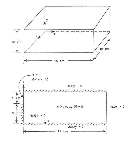
This problem concerns one-dimensional advection-dispersion of a conservative solute species through a semi-infinite porous medium (Figure 4.1). As illustrated, the contaminant is released from a channel fully penetrating a shallow confined aquifer.

An analytical solution of the problem was developed by Ogata and Banks (1961). This solution also can be found in Bear (1979). For the cases documented herein, the inlet was a first-type boundary with prescribed relative concentration of 1.0 mg/m3 . The values of Darcy velocity and effective porosity were specified as 1 m/d and 0.25, respectively. The modeled length of the aquifer domain was specified as 400 m. A uniform rectangular mesh was used consisting of 40 grid blocks, each with )x = 10 m. Three cases were studied with different values of longitudinal dispersivity ("L).

The first case had a dispersivity value of 5 m, the second case of 2 m, and the third case of zero. For the first two cases, the simulation was performed for 20 time steps with )t kept constant and equal to 2.5 days. A constant time step size of 1.25 days was used for the third case. Simulated concentration distributions using the adaptive implicit TVD scheme with the optimal time stepping are plotted in Figures 4.2, 4.3, and 4.4 at t = 50 d for the three cases

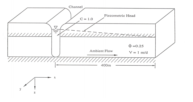
Figure 4.1 One-Dimensional Transport of a Conservative Species.

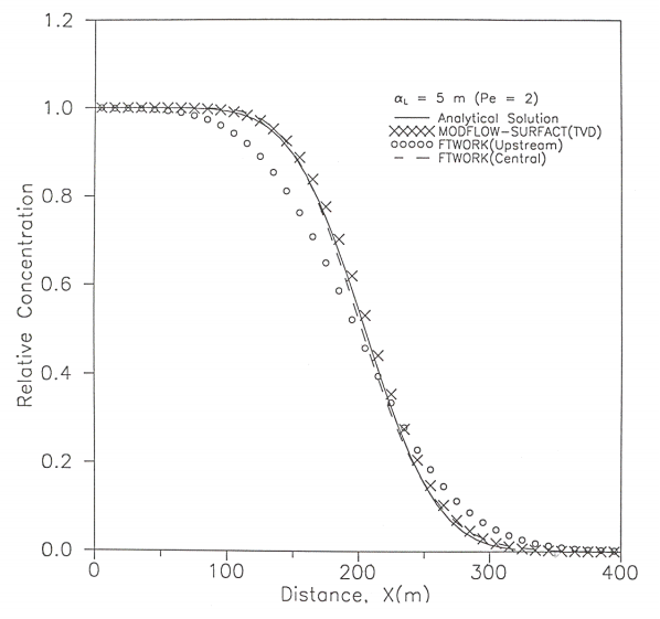
Figure 4.2 Concentration Profile at 50 Days of Simulation of Single Species One-Dimensional Transport αL=5 m (Pe=2).

Figure 4.3 Concentration Profile at 50 Days of Simulation of Single Species One-Dimensional Transport αL=2 m (Pe=5).

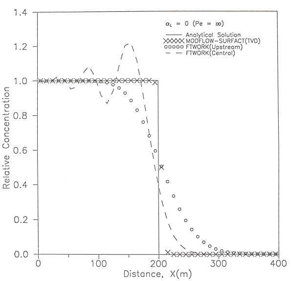
Figure 4.4 Concentration Profile at 50 Days of Simulation of Single Species One-Dimensional Transport αL=0 m (Pe=∞).

for which the grid Peclet numbers are Pe=2, 5, and 4, respectively. The grid Peclet number is defined as Pe=\Deltax/αL.

As can be seen, the numerical and analytical solutions are in excellent agreement for all cases. Upstream and central difference results obtained using FTWORK code (Faust et al, 1993) are also plotted on each of the three figures for comparison. For a low Peclet number of 2, the central difference scheme performed comparable to the TVD scheme of MODFLOW-SURFACT/MODHMS, but gave oscillatory results for higher Peclet numbers of 5 and infinity. The upstream scheme produced smeared concentration fronts for all three cases. Note that for the case of pure advection (Figure 4.4) the TVD scheme of MODFLOW-SURFACT/MODHMS was able to resolve the sharp front within 3 grid-blocks.

4.2.2 One-Dimensional Transport of a Three-Member Radioactive Decay Chain This problem is depicted schematically in Figure 4.5. The problem was selected to test implementation of the chain decay routines in MODFLOWSURFACT/MODHMS. It concerns transport of a chain of three radionuclides released from a decaying source located at x = 0 in a steady-state flow field within a confined porous medium reservoir. Analytical solutions can be found in Coats and Smith (1964) and Lester et al (1975). The flow region and the reservoir properties used in the present simulation also are depicted in Figure 4.5. The properties of the three radionuclide components and the initial and third-type decaying source boundary conditions employed are given in Table 4.1. For comparison purposes, these data were selected to correspond to the data used in a previous study on a three-member chain transport simulation reported by Reeves and Cranwell (1981). The adaptive implicit TVD scheme was selected for the simulation.

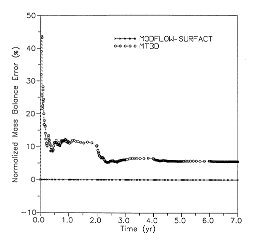
The flow region was discretized into 42 grid blocks of equal length, thus giving )x = 16.4 ft (5 m) and a mesh Peclet number Pe = 1.93. (The mesh Peclet number is defined as Pe =)x/"L.). The problem was solved for 15 time steps, with a constant time step size value of 18.26 yr. Figure 4.6 shows the concentration distributions of all three components after 273.9 years of simulation. Agreement with the analytical solution is good. Excellent mass balance results were obtained with the normalized mass balance error being less than a fraction of a percent for all three species.

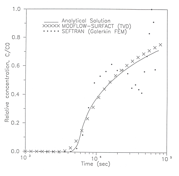
4.2.3 Transport Due to an Injection/Withdrawal Well This example problem considers an injection/pumping cycle for a fully penetrating well in a confined aquifer with zero ambient flow field (Figure 4.7).

Water of a constant concentration (C@) is injected into the well in the center of the domain for the first stress period. For the second stress period, the flow is reversed, and the contaminated groundwater is pumped out. The flow field is assumed to reach a steady state instantaneously for each stress period. An approximate analytical solution for this problem is given by Gelhar and Collins (1971).

A numerical model consisting of 31 columns, 31 rows, and 1 layer was used to simulate the concentration change at the injection/extraction well for comparison with the solution of Gelhar and Collins (1971). An axi-symmetric simulation with a refined grid at the vicinity of the well was also performed to test this option of the code.

Model parameters used in the simulation are provided in Table 4.2. A constant head of 50 ft was supplied along the outer boundary of the domain to produce a steady-state flow field. The first stress period was divided into 10 equal time steps, and the second stress period was divided into 28 equal time steps. The input data used for the MODFLOW-SURFACT/MODHMS simulation are presented in Appendix A. The adaptive implicit TVD scheme was used to solve the problem.

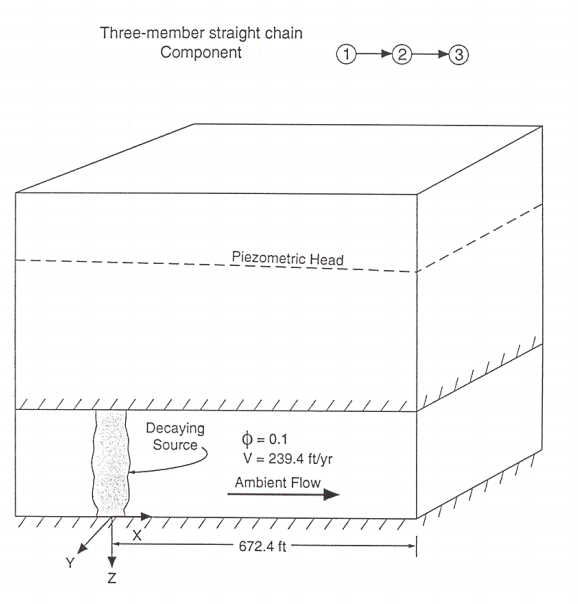
Figure 4.5 One-Dimensional Transport of a Three-Member Radioactive Decay Chain.

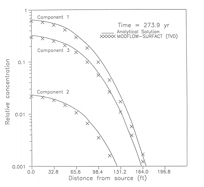
Figure 4.6 Species Concentration Distributions Showing a Comparison of Analytical and MODFLOW-SURFACT/MODHMS Solutions for One-Dimensional Transport of a Three-Member Radioactive Decay Chain.

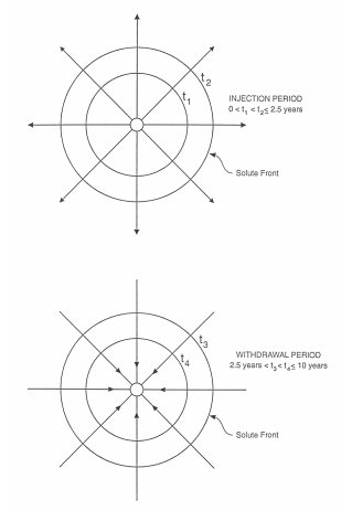
Figure 4.7 Transport Due to an Injection/Withdrawal Well.

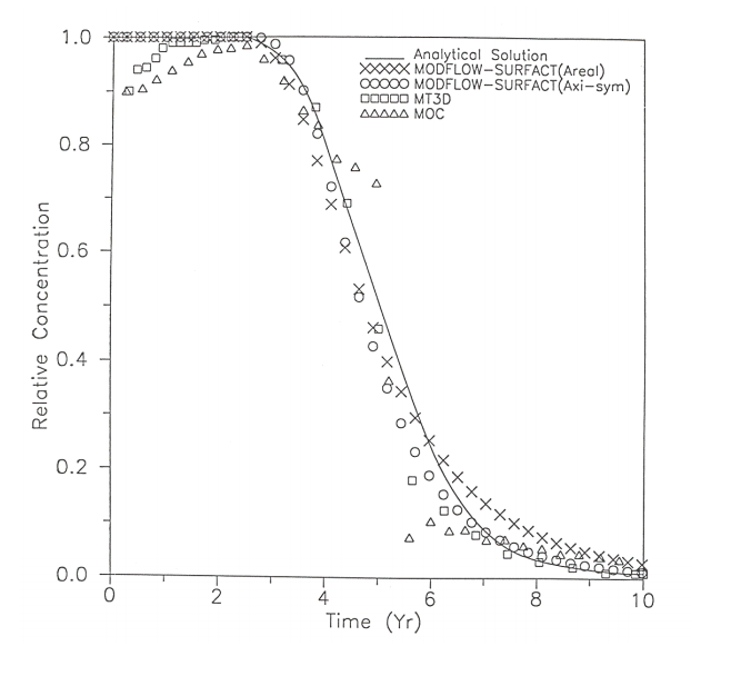
Figure 4.8 Breakthrough Curve from Simulation of Transport Due to an Injection/Withdrawal Well.

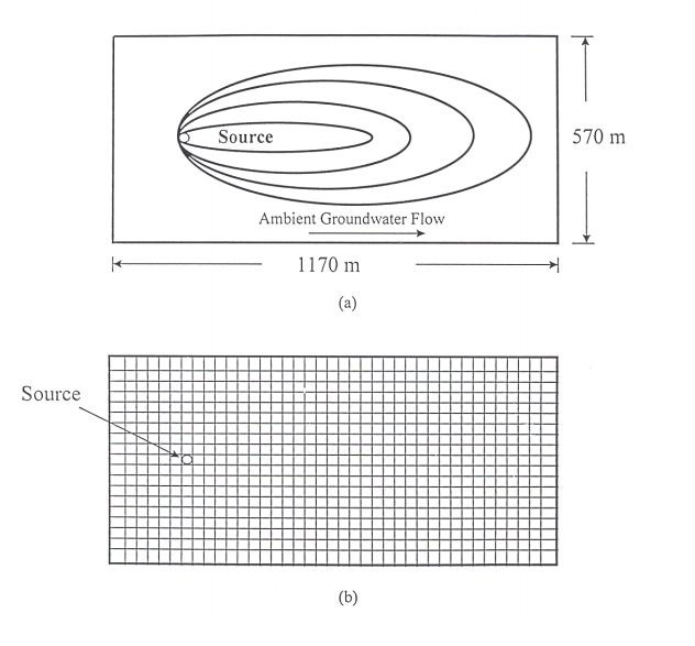
Figure 4.9 Two-Dimensional Transport from a Point Source in a Uniform Flow Field: (a) Problem Description, and (b) Model Discretization.

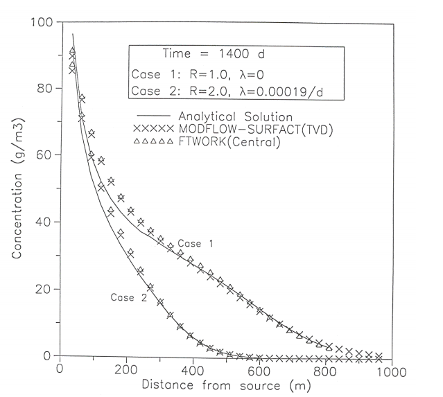
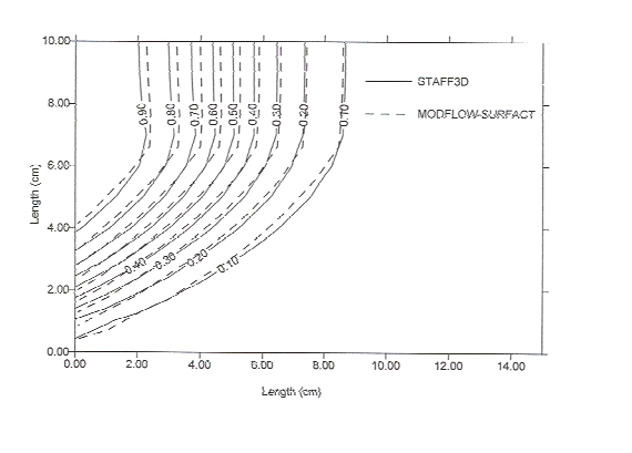
Figure 4.10 Concentration Profiles Along the Center Line of the Plume Obtained from Simulation of Two-Dimensional Transport from a Point Source in a Steady Uniform Flow Field

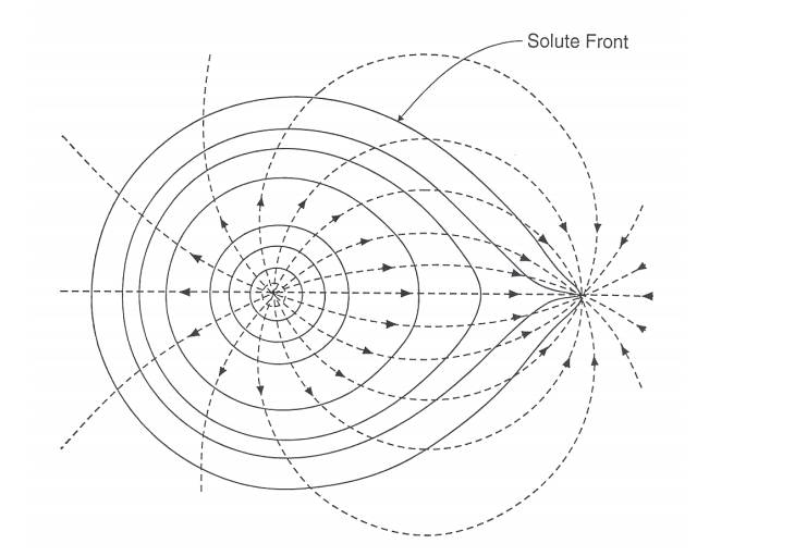
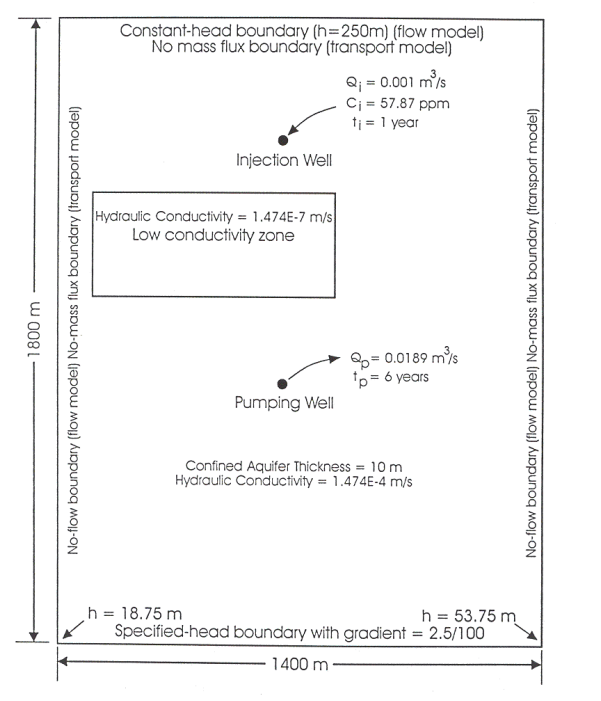
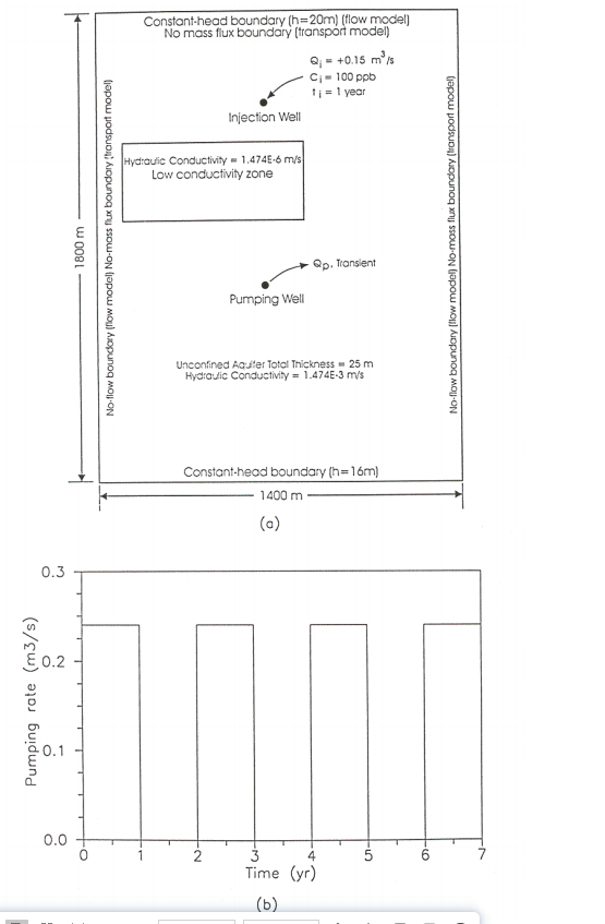
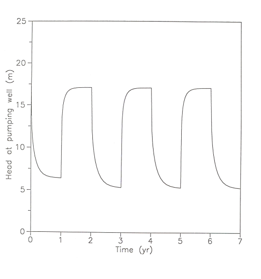
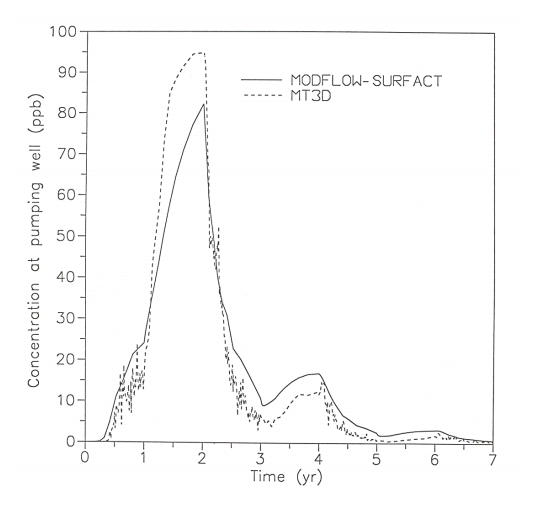
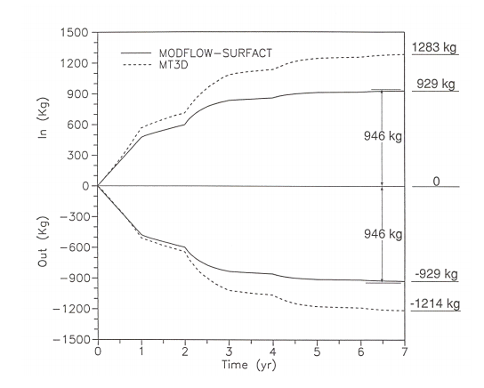
Figure 4.11 Problem Description of Transport Due to an Injection-Withdrawal Well Pair.