机器学习(十二)——感知器算法

感知器算法是一种可以直接得到线性判别函数的线性分类方法，它是基于样本线性可分的要求下使用的

---

线性可分与线性不可分

---

算法流程

感知器作为人工神经网络中最基本的单元，有多个输入和一个输出组成。虽然我们的目的是学习很多神经单元互连的网络，但是我们还是需要先对单个的神经单元进行研究。
感知器算法的主要流程：

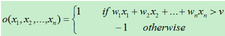
首先得到n个输入，再将每个输入值加权，然后判断感知器输入的加权和最否达到某一阀值v，若达到，则通过sign函数输出1，否则输出-1。

为了统一表达式，我们将上面的阀值v设为0，新增变量x₀=1,这样就可以使用w₀x₀+w₁x₁+w₂x₂+…+w_nx_n。于是有：

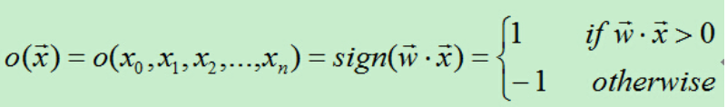
从上面的公式可知，当权值向量确定时，就可以利用感知器来做分类。

那么我们如何获得感知器的权值呢？这需要根据训练集是否可分来采用不同的方法：

1、训练集线性可分时 --> 感知器训练法则

为了得到可接受的权值，通常从随机的权值开始，然后利用训练集反复训练权值，最后得到能够正确分类所有样例的权向量。

具体算法过程如下：

A）初始化权向量w=(w₀,w₁,…,w_n)，将权向量的每个值赋一个随机值。
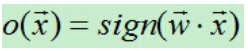
B）对于每个训练样例，首先计算其预测输出：

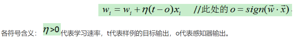
C）当预测值不等于真实值时则利用如下公式修改权向量：

D）重复B）和C），直到训练集中没有被错分的样例。

算法分析：

若某个样例被错分了，假如目标输出t为-1，结果感知器o输出为1，此时为了让感知器输出-1，需要将wx减小以输出-1，而在x的值不变的情况下只能减小w的值，这时通过在原来w后面添加(t-o)x=即可减小w的值（t-o<0, x>0）。

通过逐步调整w的值，最终感知器将会收敛到能够将所有训练集正确分类的程度，但前提条件是训练集线性可分。若训练集线性不可分，则上述过程不会收敛，将无限循环下去。

---

实现算法

1. 生成数据

import numpy as np
import matplotlib.pyplot as plt
from sklearn import datasets

iris = datasets.load_iris()

x = iris.data
y = iris.target
# 只做一个简单的二分类
x = x[y<2, :2]
y = y[y<2]

plt.scatter(x[y==0, 0], x[y==0, 1])
plt.scatter(x[y==1, 0], x[y==1, 1])
plt.show()

2. 实现算法

def check(w, x, y):
    return ((w.dot(x.T)>0).astype(int)==y).all() 

def train(w, train_x, train_y, learn=1, max_iter=200):
    iter = 0
    while ~check(w, train_x, train_y) and iter<=max_iter:
        iter += 1
        for i in range(train_y.size):
            predict_y = (w.dot(train_x[i].T)>0).astype(int)
            if predict_y != train_y[i]:
                w += learn*(train_y[i] - predict_y)*train_x[i]
    return w

def normalize(x):
    max_x = np.max(x, axis=0)
    min_x = np.min(x, axis=0)
    norm_x = (max_x - x) / (max_x - min_x)
    return norm_x

norm_x = normalize(x)
train_x = np.insert(norm_x, 0, values=np.ones(100).T, axis=1)
w = np.random.random(3)
w = train(w, train_x, y)

3. 绘制决策边界

def plot_decision_boundary(w, axis):
    x0, x1 = np.meshgrid(np.linspace(axis[0], axis[1], int((axis[1] - axis[0])*100)).reshape(1, -1),
                         np.linspace(axis[2], axis[3], int((axis[3] - axis[2])*100)).reshape(1, -1),)
    x_new = np.c_[x0.ravel(), x1.ravel()]
    x_new = np.insert(x_new, 0, np.ones(x_new.shape[0]), axis=1)
    y_predict = (w.dot(x_new.T)>0).astype(int)
    zz = y_predict.reshape(x0.shape)

    from matplotlib.colors import ListedColormap
    custom_cmap = ListedColormap(['#EF9A9A', '#FFF59D', '#90CAF9'])

    plt.contourf(x0, x1, zz, linewidth=5, cmap=custom_cmap)

plot_decision_boundary(w, axis=[-1, 1, -1, 1])
plt.scatter(norm_x[y==0, 0], norm_x[y==0, 1], color='red')
plt.scatter(norm_x[y==1, 0], norm_x[y==1, 1], color='blue')
plt.show()

4. 使用sklearn包完成感知器算法

from sklearn.datasets import make_classification
 
x,y = make_classification(n_samples=1000, n_features=2,n_redundant=0,n_informative=1,n_clusters_per_class=1)
 
#n_samples:生成样本的数量
 
#n_features=2:生成样本的特征数，特征数=n_informative（） + n_redundant + n_repeated
 
#n_informative：多信息特征的个数
 
#n_redundant：冗余信息，informative特征的随机线性组合
 
#n_clusters_per_class ：某一个类别是由几个cluster构成的 

#训练数据和测试数据
x_data_train = x[:800,:]
x_data_test = x[800:,:]
y_data_train = y[:800]
y_data_test = y[800:]
 
#正例和反例
positive_x1 = [x[i,0] for i in range(1000) if y[i] == 1]
positive_x2 = [x[i,1] for i in range(1000) if y[i] == 1]
negetive_x1 = [x[i,0] for i in range(1000) if y[i] == 0]
negetive_x2 = [x[i,1] for i in range(1000) if y[i] == 0]
from sklearn.linear_model import Perceptron
#定义感知机
clf = Perceptron(fit_intercept=False,shuffle=False)
#使用训练数据进行训练
clf.fit(x_data_train,y_data_train)
#得到训练结果，权重矩阵
print(clf.coef_)
#输出为：[[-0.38478876,4.41537463]]
 
#超平面的截距，此处输出为：[0.]
print(clf.intercept_)

#利用测试数据进行验证
acc = clf.score(x_data_test,y_data_test)
print(acc)
#得到的输出结果为0.98，这个结果还不错吧。
from matplotlib import pyplot as plt
#画出正例和反例的散点图
plt.scatter(positive_x1,positive_x2,c='red')
plt.scatter(negetive_x1,negetive_x2,c='blue')
#画出超平面（在本例中即是一条直线）
line_x = np.arange(-4,4)
line_y = line_x * (-clf.coef_[0][0] / clf.coef_[0][1]) - clf.intercept_
plt.plot(line_x,line_y)
plt.show()