


deepsort 算法详解
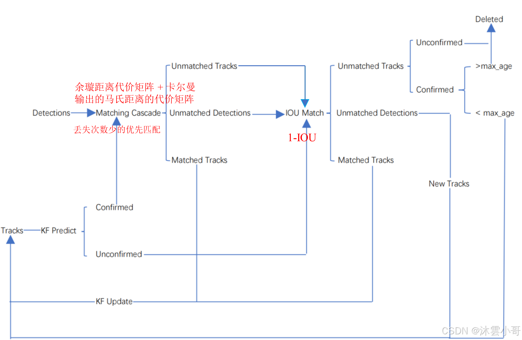
Unmatched Tracks(未匹配的轨迹)
本质角色: 是已存在的轨迹在当前帧中“失联”的状态,即预测位置与检测结果不匹配。
生命周期阶段:
已初始化: 轨迹已存在多帧,可能携带历史信息(如外观特征、运动模型)。
未被观测到: 当前帧中未找到对应的检测框,可能因遮挡、目标消失或检测漏检导致。
处理逻辑:
未匹配计数增加: 记录连续未匹配的帧数(如time_since_update)。
删除条件: 若未匹配次数超过阈值(如max_age),轨迹被删除。
预测继续: 即使未匹配,算法仍会预测下一帧的位置,以尝试重新匹配。
Unmatched Detections(未匹配的检测框)
本质角色: 是新检测到的候选目标,未被任何现有轨迹“认领”。
生命周期阶段:
- 新出现的候选: 当前帧的检测结果,尚未被关联到已有轨迹。
- 可能初始化为新轨迹:若未匹配到任何轨迹,需决定是否将其作为新轨迹的起点。
处理逻辑:
- 初始化为新轨迹:
SORT:直接初始化为新轨迹(无确认机制)。DeepSORT:需满足连续匹配次数阈值(如n_init=3)才能转为“确认态”。
- 外观特征记录:
DeepSORT会保存检测框的外观特征(如深度学习提取的向量),用于后续匹配。
| 维度 | Unmatched Tracks | Unmatched Detections |
|---|---|---|
| 本质 | 历史存在但暂时未被观测到的目标 | 新出现但未被关联到任何目标的候选 |
| 处理逻辑 | 删除或保留决策 | 初始化新轨迹或忽略 |
| 算法目标 | 保持轨迹连续性与鲁棒性 | 发现新目标与抗干扰 |
2. 卡尔曼滤波代码分析
2. 1 初始化状态转移矩阵 F F F和观测矩阵 H H H
class KalmanFilterXYAH:
    """
    A KalmanFilterXYAH class for tracking bounding boxes in image space using a Kalman filter.

    Implements a simple Kalman filter for tracking bounding boxes in image space. The 8-dimensional state space
    (x, y, a, h, vx, vy, va, vh) contains the bounding box center position (x, y), aspect ratio a, height h, and their
    respective velocities. Object motion follows a constant velocity model, and bounding box location (x, y, a, h) is
    taken as a direct observation of the state space (linear observation model).

    Attributes:
        _motion_mat (np.ndarray): The motion matrix for the Kalman filter.    F
        _update_mat (np.ndarray): The update matrix for the Kalman filter.    H
        _std_weight_position (float): Standard deviation weight for position.  标准差的权重[x  y  a  h  dx dy da dh ]
        _std_weight_velocity (float): Standard deviation weight for velocity.

    Methods:
        initiate: Creates a track from an unassociated measurement.
        predict: Runs the Kalman filter prediction step.
        project: Projects the state distribution to measurement space.
        multi_predict: Runs the Kalman filter prediction step (vectorized version).
        update: Runs the Kalman filter correction step.
        gating_distance: Computes the gating distance between state distribution and measurements.

    Examples:
        Initialize the Kalman filter and create a track from a measurement
        >>> kf = KalmanFilterXYAH()
        >>> measurement = np.array([100, 200, 1.5, 50])
        >>> mean, covariance = kf.initiate(measurement)
        >>> print(mean)
        >>> print(covariance)
    """

    def __init__(self):
        """
        Initialize Kalman filter model matrices with motion and observation uncertainty weights.

        The Kalman filter is initialized with an 8-dimensional state space (x, y, a, h, vx, vy, va, vh), where (x, y)
        represents the bounding box center position, 'a' is the aspect ratio, 'h' is the height, and their respective
        velocities are (vx, vy, va, vh). The filter uses a constant velocity model for object motion and a linear
        observation model for bounding box location.

        Examples:
            Initialize a Kalman filter for tracking:
            >>> kf = KalmanFilterXYAH()
        """

        ndim, dt = 4, 1.0

        # Create Kalman filter model matrices
        self._motion_mat = np.eye(2 * ndim, 2 * ndim)   # F[8,8]
        for i in range(ndim):
            self._motion_mat[i, ndim + i] = dt
        self._update_mat = np.eye(ndim, 2 * ndim)       # H[4,8]

        # Motion and observation uncertainty are chosen relative to the current state estimate. These weights control
        # the amount of uncertainty in the model.
        self._std_weight_position = 1.0 / 20
        self._std_weight_velocity = 1.0 / 160
ndim = 4:表示位置相关状态的数量,即 x , y , a , h x, y, a, h x,y,a,h(中心坐标、宽高比、高度)。dt = 1.0:时间步长,默认为1秒。- 状态转移矩阵
F
F
F(
_motion_mat) - 观测矩阵
H
H
H(
_update_mat),4×8的单位矩阵,仅保留前4行(对应位置和尺寸 x x x, y y y, a a a, h h h) std_weight_position:位置噪声权重(默认 0.05)。std_weight_velocity:速度噪声权重(默认 0.00625)
2.2 initiate 方法分析
initiate 方法用于根据初始观测值(未关联的检测框)创建一个新的跟踪轨迹的初始状态(均值向量和协方差矩阵)
输入: 观测值为
z
0
=
[
x
,
y
,
a
,
h
]
z_0 = [x, y, a, h]
z0=[x,y,a,h]
输出:
- 均值向量 μ 0 \mu_0 μ0: 8维(包含位置和速度的初始估计)
- 协方差矩阵 P 0 P_0 P0 :8×8维,表示初始状态的不确定性均值向量。
   def initiate(self, measurement: np.ndarray) -> tuple:
        """
        Create a track from an unassociated measurement.

        Args:
            measurement (ndarray): Bounding box coordinates (x, y, a, h) with center position (x, y), aspect ratio a,
                and height h.

        Returns:
            (tuple[ndarray, ndarray]): Returns the mean vector (8-dimensional) and covariance matrix (8x8 dimensional)
                of the new track. Unobserved velocities are initialized to 0 mean.

        Examples:
            >>> kf = KalmanFilterXYAH()
            >>> measurement = np.array([100, 50, 1.5, 200])
            >>> mean, covariance = kf.initiate(measurement)   # x_k,  p_k
        """
        mean_pos = measurement               # [4,] [x, y, a, h]
        mean_vel = np.zeros_like(mean_pos)   # [4,] [0, 0, 0, 0]
        mean = np.r_[mean_pos, mean_vel]     # [8,]  np.r_[] 按行放在一起    [100,50,1.5,200,0,0,0,0]

        std = [
            2 * self._std_weight_position * measurement[3], 	# x 方向
            2 * self._std_weight_position * measurement[3], 	# y 方向
            1e-2,												# a
            2 * self._std_weight_position * measurement[3], 	# h方向
            10 * self._std_weight_velocity * measurement[3],	# v_x
            10 * self._std_weight_velocity * measurement[3],	# v_y
            1e-5,												# v_a
            10 * self._std_weight_velocity * measurement[3],	# v_h
        ]   # [20.0, 20.0, 0.01, 20.0, 12.5, 12.5, 1e-05, 12.5]
        covariance = np.diag(np.square(std))    # [8,8] 对角矩阵  [20^2, 20^2 , 0.01^2, 20^2, 12.5^2, 12.5^2, (1e−5)^2, 12.5^2]
        return mean, covariance                 # (8,), (8, 8)
2.3 predict方法分析
predict方法实现了卡尔曼滤波的预测步骤,通过状态转移矩阵
F
\mathbf{F}
F 和过程噪声协方差
Q
\mathbf{Q}
Q 对下一时刻的状态进行预测,得到预测结果下的均值(mean)和协方差(covariance)。
- 计算下一时刻的均值(位置 = 当前位置 + 速度)。
- 更新协方差矩阵,结合状态转移和过程噪声。
- 假设宽高比变化极小,速度噪声较低,确保滤波的鲁棒性。
def predict(self, mean: np.ndarray, covariance: np.ndarray) -> tuple:
        """
        Run Kalman filter prediction step.

        Args:
            mean (ndarray): The 8-dimensional mean vector of the object state at the previous time step.
            covariance (ndarray): The 8x8-dimensional covariance matrix of the object state at the previous time step.

        Returns:
            (tuple[ndarray, ndarray]): Returns the mean vector and covariance matrix of the predicted state. Unobserved
                velocities are initialized to 0 mean.

        Examples:    x_k+1 = F* x_k  ; P_K+1 = F* p_k * F^T
            >>> kf = KalmanFilterXYAH()
            >>> mean = np.array([0, 0, 1, 1, 0, 0, 0, 0])
            >>> covariance = np.eye(8)
            >>> predicted_mean, predicted_covariance = kf.predict(mean, covariance)
        """
        # 位置和速度的标准差 self._std_weight_position:权重 mean[3] 指的是状态向量中的高度
        std_pos = [
            self._std_weight_position * mean[3],
            self._std_weight_position * mean[3],
            1e-2,
            self._std_weight_position * mean[3],
        ]     # [0.05, 0.05, 0.01, 0.05]
        std_vel = [
            self._std_weight_velocity * mean[3],
            self._std_weight_velocity * mean[3],
            1e-5,
            self._std_weight_velocity * mean[3],
        ]    # [0.00625, 0.00625, 1e-05, 0.00625]
        motion_cov = np.diag(np.square(np.r_[std_pos, std_vel]))   # Q_k (8, 8)
        """
        		x_k+1 = F * x_k
        		x_k 为 k时刻的均值,F称为状态转移矩阵, 该公式预测k+1时刻的 x_k+1时刻的均值
        		self._motion_mat F作用在x_k上的状态变换模型
        """
        mean = np.dot(mean, self._motion_mat.T)
        """
        		p_K+1 = F* p_k * F^T +Q_k
        		P_k 为 k时刻的协方差,Q_k 为k时刻的噪声矩阵,代表整个系统可靠程度。
        		预测 k+1时刻的协方差
        """
        covariance = np.linalg.multi_dot((self._motion_mat, covariance, self._motion_mat.T)) + motion_cov # 协方差更新 按顺序计算三个矩阵的乘积,确保矩阵乘法的正确性

        return mean, covariance
卡尔曼滤波的预测方程:
x
^
k
+
1
=
F
x
^
k
+
B
u
k
\hat{\mathbf{x}}_{k+1} = \mathbf{F} \hat{\mathbf{x}}_{k} + \mathbf{B} \mathbf{u}_{k}
x^k+1=Fx^k+Buk
P
^
k
+
1
=
F
⋅
P
^
k
F
⊤
+
Q
\hat{\mathbf{P}}_{k+1} = F \cdot \hat{\mathbf{P}}_{k} F^\top + Q
P^k+1=F⋅P^kF⊤+Q
- P k \mathbf{P_k} Pk: x k x_k xk的方差
- F \mathbf{F} F:状态转移矩阵(self._motion_mat)
- Q \mathbf{Q} Q:过程噪声协方差矩阵(motion_cov)
2.4 project() 方法分析
该函数将状态空间的预测状态(均值和协方差)投影到测量空间,返回预测的测量值及其协方差。这是卡尔曼滤波测量阶段的关键步骤。
    def project(self, mean: np.ndarray, covariance: np.ndarray) -> tuple:
        """  通过状态值x估计观测值Z
        Project state distribution to measurement space.

        Args:
            mean (ndarray): The state's mean vector (8 dimensional array).
            covariance (ndarray): The state's covariance matrix (8x8 dimensional).

        Returns:
            (tuple[ndarray, ndarray]): Returns the projected mean and covariance matrix of the given state estimate.

        Examples:
            >>> kf = KalmanFilterXYAH()
            >>> mean = np.array([0, 0, 1, 1, 0, 0, 0, 0])
            >>> covariance = np.eye(8)
            >>> projected_mean, projected_covariance = kf.project(mean, covariance)
        """
        std = [
            self._std_weight_position * mean[3],		# x坐标噪声标准差(与高度相关)
            self._std_weight_position * mean[3],		# y坐标噪声标准差(与高度相关)
            1e-1,										# 宽高比噪声标准差(固定值)
            self._std_weight_position * mean[3],		# 高度噪声标准差(与高度相关)
        ]    # [0.05, 0.05, 0.1, 0.05]
        innovation_cov = np.diag(np.square(std))    # R_k [4,4]

        mean = np.dot(self._update_mat, mean)       # _update_mat(H)    x'_k = H * x_k  [4,] 观测值Zk的估计值
        covariance = np.linalg.multi_dot((self._update_mat, covariance, self._update_mat.T))  #  P'_k = H * p_k * H.T  观测值Zk的方差
        return mean, covariance + innovation_cov    # (4, 4)
2.5 update()方法分析
代码主题思想解释:
卡尔曼滤波的测量更新步骤,根据以下公式求得新的卡尔曼增益值、均值、协方差,最后返回更新后的均值和协方差。
卡尔曼更新方程:
k
∗
=
P
k
^
H
k
T
(
H
k
P
k
^
H
k
T
+
R
k
)
−
1
(
1
)
\mathbf{k}^* = \hat{\mathbf{P}_{k}} \mathbf{H}_{k}^T (\mathbf{H}_{k}\hat{\mathbf{P}_{k}}\mathbf{H}_{k}^T + \mathbf{R}_{k})^{-1} (1)
k∗=Pk^HkT(HkPk^HkT+Rk)−1(1)
x k ∗ ^ = k ∗ ( z k − H k x k ^ ) ( 2 ) \hat{\mathbf{x}_{k}^*} = \mathbf{k}^* (\mathbf{z}_{k} - \mathbf{H}_{k}\hat{\mathbf{x}_{k}}) (2) xk∗^=k∗(zk−Hkxk^)(2)
P k ∗ ^ = P k ^ − k ∗ H k P k ^ ( 3 ) \hat{\mathbf{P}_{k}^*} = \hat{\mathbf{P}_{k}} - \mathbf{k}^*\mathbf{H}_{k}\hat{\mathbf{P}_{k}} (3) Pk∗^=Pk^−k∗HkPk^(3)
    def update(self, mean: np.ndarray, covariance: np.ndarray, measurement: np.ndarray) -> tuple:
        """
        Run Kalman filter correction step.

        Args:
            mean (ndarray): The predicted state's mean vector (8 dimensional).
            covariance (ndarray): The state's covariance matrix (8x8 dimensional).
            measurement (ndarray): The 4 dimensional measurement vector (x, y, a, h), where (x, y) is the center
                position, a the aspect ratio, and h the height of the bounding box.

        Returns:
            (tuple[ndarray, ndarray]): Returns the measurement-corrected state distribution.

        Examples:
            >>> kf = KalmanFilterXYAH()
            >>> mean = np.array([0, 0, 1, 1, 0, 0, 0, 0])   x_k
            >>> covariance = np.eye(8)                      p_k
            >>> measurement = np.array([1, 1, 1, 1])        z_k
            >>> new_mean, new_covariance = kf.update(mean, covariance, measurement)
        """
        projected_mean, projected_cov = self.project(mean, covariance)  # H_k*x_k ; H_k*P_k*H_k.T+R_k
        # 用矩阵分解求卡尔曼增益
        chol_factor, lower = scipy.linalg.cho_factor(projected_cov, lower=True, check_finite=False)
        kalman_gain = scipy.linalg.cho_solve(
            (chol_factor, lower), np.dot(covariance, self._update_mat.T).T, check_finite=False
        ).T   # k^*  ;covariance(P_k) ; _update_mat(H_k)
        innovation = measurement - projected_mean                  # z_k - H_k * x_k

        new_mean = mean + np.dot(innovation, kalman_gain.T)        # x' = x_k+ K^* *(z_k - H_k * x_k)
        new_covariance = covariance - np.linalg.multi_dot((kalman_gain, projected_cov, kalman_gain.T))  #  P' = P_k- K^* * H_k * P_k)
        return new_mean, new_covariance
3. 匈牙利算法
3.1 原理
匈牙利算法基于代价矩阵找到最小代价的分配方法,是解决分配问题中最优匹配(最小代价)的算法。
3.2 依据
代价矩阵的行或列同时加或减一个数,得到新的代价矩阵的最优匹配与原代价矩阵相同
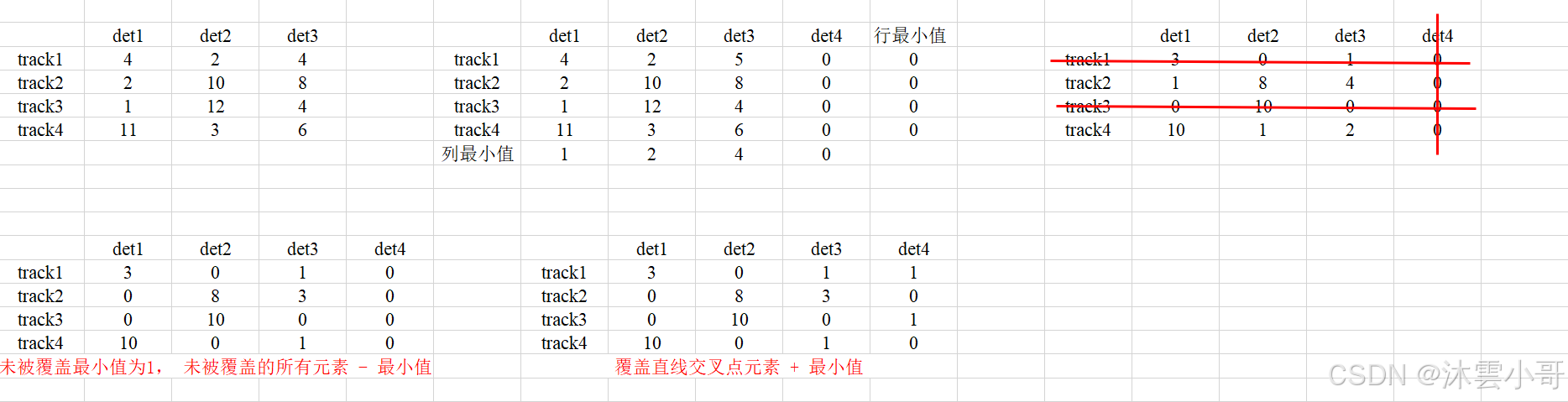
3.3 步骤
(1)如果代价矩阵不为方阵,则在相应位置补0使得代价矩阵为方阵。
(2)首先代价矩阵每一行减去此行最小值,每一列减去此列最小值。
(3)用最少的横线或竖线覆盖代价矩阵中的所有0元素。
(4)如果线的条数小于方阵维数,找出步骤3中未被覆盖元素的最小值,且未被覆盖元素减去该最小值;对覆盖直线交叉点元素加上该最小值。
(5)重复步骤(3)、(4),直到覆盖线的数量等于对应方阵的维度数。
(6)当线的条数等于方阵维数时,从行或列中找0数最小的匹配对,以此类推,找到所有匹配的行和列。
3.4 步骤图
追踪流程拆解:
-
第一帧:
(1) 假设检测有10 个bbox,此时由于是第一帧因此没有track。
(2) 因为没有track,因此不会执行任何deepsort追踪。
(3) 对当前10个检测结果分别初始化track。 -
第二帧:
(1)假设检测有11个bbox,进行IOU匹配(级联匹配需要confirmed track,需要三帧命中)。
(2)此时匹配到10个track,将匹配到的更新每一个track卡尔曼参数。
(3)有一个预测的bbox未能匹配上,则需要New track。 -
第三帧:
(1)假设检测有12个bbox,当前还是没有confirm的track (需要三帧命中)
(2)前面创建的11个track要继续与12个bbox进行IOU匹配
(3)若其中有一个track没有匹配上(此时是unconfirmed状态)则将这个track删除
(4)其中有10个track已经命中三次,则需要将这些track状态更新为confirm -
第四帧:
(1)假设检测有14个bbox, 不仅要做IOU匹配 ,还要做级联匹配
(2)对前面10个confirm的track进行级联匹配(优先) ,然后在进行IOU匹配
(3)每次匹配到的track都要更新其卡尔曼参数
追踪流程拆解总结:
- 检测得到当前帧的bbox(其实追踪好坏主要取决于检测结果)。
- track分为:confirmed和unconfirmed 两者待遇不同。
- 对于confirmed要先进行级联匹配,它们优先级高,连续70帧没有匹配上会删除。
- 代价矩阵包括Reid特征构建的余弦距离与运动信息构建的马氏距离。
- 对于级联匹配玩剩下的和当前是unconfirmed与剩下的bbox进行IOU匹配。
- 经过级联与IOU匹配后就得到了所有匹配结果,要更新track参数。
- 对于匹配成功的track,连续命中3次以上才能转换成confirmed。
- 对于没有匹配成功的track,如果他是unconfirmed则删除。
DeepSORT代码中update方法是目标跟踪系统的核心函数,负责:
特征提取: 从检测到的目标中提取外观特征(如ReID特征)。
预处理检测结果: 筛选低置信度检测并执行非极大值抑制(NMS)。
跟踪更新: 通过卡尔曼滤波预测和匈牙利算法匹配,更新目标轨迹。
结果输出: 整理跟踪结果为边界框和唯一ID。
    def update(self, bbox_xywh, confidences, ori_img):
        self.height, self.width = ori_img.shape[:2]
        # generate detections
        # 从原图中抠取bbox对应图片并计算得到相应的特征
        features = self._get_features(bbox_xywh, ori_img)
        bbox_tlwh = self._xywh_to_tlwh(bbox_xywh)
        # 筛选掉小于min_confidence的目标,并构造一个Detection对象构成的列表 [坐标,置信度,特征]
        detections = [Detection(bbox_tlwh[i], conf, features[i]) for i,conf in enumerate(confidences) if conf>self.min_confidence]

        # run on non-maximum supression
        boxes = np.array([d.tlwh for d in detections])
        scores = np.array([d.confidence for d in detections])
        indices = non_max_suppression(boxes, self.nms_max_overlap, scores)
        detections = [detections[i] for i in indices]

        # update tracker
        self.tracker.predict() # 将跟踪状态分布向前传播一步
        self.tracker.update(detections) # 执行测量更新和跟踪管理

        # output bbox identities
        outputs = []
        for track in self.tracker.tracks:
            if not track.is_confirmed() or track.time_since_update > 1:
                continue
            box = track.to_tlwh()
            x1,y1,x2,y2 = self._tlwh_to_xyxy(box)
            track_id = track.track_id
            outputs.append(np.array([x1,y1,x2,y2,track_id], dtype=np.int))
        if len(outputs) > 0:
            outputs = np.stack(outputs,axis=0)
        return outputs
抠图部分进行特征提取
    # 获取抠图部分的特征
    def _get_features(self, bbox_xywh, ori_img):
        im_crops = []
        for box in bbox_xywh:
            x1,y1,x2,y2 = self._xywh_to_xyxy(box)
            # x1, y1, x2, y2从原始图像ori_img中裁剪出对应的目标区域im
            im = ori_img[y1:y2,x1:x2] # 抠图部分
            im_crops.append(im)
        if im_crops:
        	# 调用特征提取器 卷积+池化构成的网络
            features = self.extractor(im_crops)
        else:
            features = np.array([])
        return features
更新卡尔曼增益以及匈牙利匹配:
- 将当前帧的检测结果(detections)与现有跟踪轨迹(tracks)进行匹配。
- 根据匹配结果更新轨迹状态
- 删除无效轨迹(如长时间未匹配),初始化新轨迹。
- 利用当前有效轨迹的特征更新外观相似度模型(如余弦距离度量)
tracker.py -> self.tracker.update(detections)
 def update(self, detections):
        """Perform measurement update and track management.
        执行测量更新和轨迹管理
        Parameters
        ----------
        detections : List[deep_sort.detection.Detection]
            A list of detections at the current time step.
        """
        # Run matching cascade.
        matches, unmatched_tracks, unmatched_detections = \
            self._match(detections)

        # Update track set.
        """
        	更新卡尔曼参数,以及最终的detection
        """
        # 1. 针对匹配上的结果
        for track_idx, detection_idx in matches:
            # 更新tracks中相应的detection
            self.tracks[track_idx].update(
                self.kf, detections[detection_idx])

        # 2. 针对未匹配的track, 调用mark_missed进行标记
        # track失配时,若Tantative则删除;若update时间很久也删除
        for track_idx in unmatched_tracks:
            self.tracks[track_idx].mark_missed()

        # 3. 针对未匹配的detection, detection失配,进行初始化
        for detection_idx in unmatched_detections:
            self._initiate_track(detections[detection_idx])

        # 得到最新的tracks列表,保存的是标记为Confirmed和Tentative的track
        self.tracks = [t for t in self.tracks if not t.is_deleted()]

        # Update distance metric.
        active_targets = [t.track_id for t in self.tracks if t.is_confirmed()]
        features, targets = [], []
        for track in self.tracks:
            # 获取所有Confirmed状态的track id
            if not track.is_confirmed():
                continue
            features += track.features # 将Confirmed状态的track的features添加到features列表
            # 获取每个feature对应的trackid
            targets += [track.track_id for _ in track.features]
            track.features = []
        # 距离度量中的特征集更新
        self.metric.partial_fit(
            np.asarray(features), np.asarray(targets), active_targets)
初始化track
# 一般第一帧需要初始化track
def _initiate_track(self, detection):
        mean, covariance = self.kf.initiate(detection.to_xyah())
        self.tracks.append(Track(
            mean, covariance, self._next_id, self.n_init, self.max_age,
            detection.feature))
        self._next_id += 1
    def predict(self, kf):
        """Propagate the state distribution to the current time step using a
        Kalman filter prediction step.
        使用卡尔曼滤波器预测步骤将状态分布传播到当前时间步

        Parameters
        ----------
        kf : kalman_filter.KalmanFilter
            The Kalman filter.

        """
        # 更新轨迹的均值(mean)和协方差(covariance)
        # mean:预测的下一帧目标状态(包含位置、速度等)
        # age 表示轨迹的总存活时间(每帧递增), covariance:预测状态的不确定性(协方差矩阵)
		# time_since_update 表示自上次匹配成功的未匹配时间(仅在未匹配时递增)
        self.mean, self.covariance = kf.predict(self.mean, self.covariance)
        self.age += 1
        self.time_since_update += 1
mean和covariance的计算代码(轨迹预测)
- 状态转移矩阵。
- 根据状态转移矩阵获取下一状态和其协方差。
kalman_filter.py -> self.tracker.predict() –> track.predict(self.kf) –> def predict(self, mean, covariance)
    def predict(self, mean, covariance):
        """Run Kalman filter prediction step.

        Parameters
        ----------
        mean : ndarray
        	x, y, a, h, vx, vy, va, vh
            The 8 dimensional mean vector of the object state at the previous
            time step.
        covariance : ndarray
            The 8x8 dimensional covariance matrix of the object state at the
            previous time step.

        Returns
        -------
        (ndarray, ndarray)
            Returns the mean vector and covariance matrix of the predicted
            state. Unobserved velocities are initialized to 0 mean.

        """
        #卡尔曼滤波器由目标上一时刻的均值和协方差进行预测。
        std_pos = [
            self._std_weight_position * mean[3],
            self._std_weight_position * mean[3],
            1e-2,
            self._std_weight_position * mean[3]]
        std_vel = [
            self._std_weight_velocity * mean[3],
            self._std_weight_velocity * mean[3],
            1e-5,
            self._std_weight_velocity * mean[3]]

        # 初始化噪声矩阵Q;np.r_ 按列连接两个矩阵
        # motion_cov是过程噪声 W_k的 协方差矩阵Qk
        motion_cov = np.diag(np.square(np.r_[std_pos, std_vel]))

        # Update time state x' = Fx (1)
        # x为track在t-1时刻的均值,F称为状态转移矩阵,该公式预测t时刻的x'
        # self._motion_mat为F_k是作用在 x_{k-1}上的状态变换模型
        mean = np.dot(self._motion_mat, mean)
        # Calculate error covariance P' = FPF^T+Q (2)
        # P为track在t-1时刻的协方差,Q为系统的噪声矩阵,代表整个系统的可靠程度,一般初始化为很小的值,
        # 该公式预测t时刻的P'
        covariance = np.linalg.multi_dot((
            self._motion_mat, covariance, self._motion_mat.T)) + motion_cov

        return mean, covariance
轨迹与特征匹配
轨迹与特征匹配步骤:
- 把轨迹分为确认状态和非确认状态。 级联匹配。
- 如果是确认状态,则需要进行级联匹配,通过级联匹配得到匹配的tracks_id(matches_a)、未匹配的tracks(unmatched_tracks_a)、未匹配检测(unmatched_detections)。
- IOU匹配。把级联匹配步骤中只有一次未匹配的轨迹并且非确认状态轨迹用于IOU匹配;
- 保留级联匹配步骤中未匹配的轨迹中连续2帧或2帧以上没有匹配的轨迹。
- 更新级联匹配和IOU匹配的结果。
    def _match(self, detections):

        def gated_metric(tracks, dets, track_indices, detection_indices):
            features = np.array([dets[i].feature for i in detection_indices])   # 检测框的特征
            targets = np.array([tracks[i].track_id for i in track_indices])     # 轨迹的id
            cost_matrix = self.metric.distance(features, targets)               # 计算轨迹与检测的特征余弦距离
            cost_matrix = linear_assignment.gate_cost_matrix(                   # 用轨迹与检测的马氏距离跟新cost_matrix矩阵
                self.kf, cost_matrix, tracks, dets, track_indices,
                detection_indices)

            return cost_matrix

        # Split track set into confirmed and unconfirmed tracks.
        # 1 把轨迹分为确认状态和非确认状态
        confirmed_tracks = [
            i for i, t in enumerate(self.tracks) if t.is_confirmed()]
        unconfirmed_tracks = [
            i for i, t in enumerate(self.tracks) if not t.is_confirmed()]

        # Associate confirmed tracks using appearance features.
        # 2 级联匹配
        matches_a, unmatched_tracks_a, unmatched_detections = \
            linear_assignment.matching_cascade(
                gated_metric, self.metric.matching_threshold, self.max_age,
                self.tracks, detections, confirmed_tracks)

        # Associate remaining tracks together with unconfirmed tracks using IOU.
        # 3 IOU匹配
        iou_track_candidates = unconfirmed_tracks + [
            k for k in unmatched_tracks_a if
            self.tracks[k].time_since_update == 1]   # 如果级联未匹配轨迹上一帧匹配成功,这一帧匹配失败,则把其添加到不确认轨迹中
        unmatched_tracks_a = [
            k for k in unmatched_tracks_a if
            self.tracks[k].time_since_update != 1]   # 跟新unmatched_tracks_a,只保留大于等于连续两帧没有被匹配上的
        matches_b, unmatched_tracks_b, unmatched_detections = \
            linear_assignment.min_cost_matching(
                iou_matching.iou_cost, self.max_iou_distance, self.tracks,
                detections, iou_track_candidates, unmatched_detections)  # IOU匹配
        # 4 更新级联匹配和IOU匹配的结果
        matches = matches_a + matches_b
        unmatched_tracks = list(set(unmatched_tracks_a + unmatched_tracks_b))
        return matches, unmatched_tracks, unmatched_detections

    def _initiate_track(self, detection):
        mean, covariance = self.kf.initiate(detection.to_xyah()) # 根据新检测到的框初始化轨迹的数值和协方差
        self.tracks.append(Track(
            mean, covariance, self._next_id, self.n_init, self.max_age,detection.oid,
            detection.feature))               # 添加新的轨迹
        self._next_id += 1

# 2 级联匹配
 """
 级联匹配优先匹配track[tarck1, track2, ................]中丢失匹配帧数少的,比如:track1匹配丢失1帧,track2匹配丢失10帧,那么就需要优先track1 与 det进行匹配。
 """
级联匹配步骤:
2.1 获取(1 + level)次没有被匹配上的轨迹
2.2 计算轨迹特征和检测特征的代价矩阵
    2.2.1 计算轨迹与检测的特征余弦距离
    2.2.2 用轨迹与检测的马氏距离跟新cost_matrix矩阵

def matching_cascade(
        distance_metric, max_distance, cascade_depth, tracks, detections,
        track_indices=None, detection_indices=None):
    """Run matching cascade.

    Parameters
    ----------
    distance_metric : Callable[List[Track], List[Detection], List[int], List[int]) -> ndarray
        The distance metric is given a list of tracks and detections as well as
        a list of N track indices and M detection indices. The metric should
        return the NxM dimensional cost matrix, where element (i, j) is the
        association cost between the i-th track in the given track indices and
        the j-th detection in the given detection indices.
    max_distance : float
        Gating threshold. Associations with cost larger than this value are
        disregarded.
    cascade_depth: int
        The cascade depth, should be se to the maximum track age.
    tracks : List[track.Track]
        A list of predicted tracks at the current time step.
    detections : List[detection.Detection]
        A list of detections at the current time step.
    track_indices : Optional[List[int]] 轨迹ID
        List of track indices that maps rows in `cost_matrix` to tracks in
        `tracks` (see description above). Defaults to all tracks.
    detection_indices : Optional[List[int]] 检测框ID
        List of detection indices that maps columns in `cost_matrix` to
        detections in `detections` (see description above). Defaults to all
        detections.

    Returns
    -------
    (List[(int, int)], List[int], List[int])
        Returns a tuple with the following three entries:
        * A list of matched track and detection indices.
        * A list of unmatched track indices.
        * A list of unmatched detection indices.

    """
    if track_indices is None:
        track_indices = list(range(len(tracks)))
    if detection_indices is None:
        detection_indices = list(range(len(detections)))

    unmatched_detections = detection_indices              # 初始所有的检测都没有匹配
    matches = []
    for level in range(cascade_depth):
        if len(unmatched_detections) == 0:                # No detections left
            break
        # 1 获取(1 + level)次没有被匹配上的轨迹
        track_indices_l = [
            k for k in track_indices
            if tracks[k].time_since_update == 1 + level
        ]
        if len(track_indices_l) == 0:                     # Nothing to match at this level
            continue
        # 2 计算轨迹特征和检测特征的马氏距离
        matches_l, _, unmatched_detections = \
            min_cost_matching(
                distance_metric, max_distance, tracks, detections,  # max_distance阈值
                track_indices_l, unmatched_detections)
        matches += matches_l
    unmatched_tracks = list(set(track_indices) - set(k for k, _ in matches))
    return matches, unmatched_tracks, unmatched_detections
用轨迹与检测的马氏距离跟新cost_matrix矩阵
def gate_cost_matrix(
        kf, cost_matrix, tracks, detections, track_indices, detection_indices,
        gated_cost=INFTY_COST, only_position=False):
    """Invalidate infeasible entries in cost matrix based on the state
    distributions obtained by Kalman filtering.

    Parameters
    ----------
    kf : The Kalman filter.
    cost_matrix : ndarray
        The NxM dimensional cost matrix, where N is the number of track indices
        and M is the number of detection indices, such that entry (i, j) is the
        association cost between `tracks[track_indices[i]]` and
        `detections[detection_indices[j]]`.
    tracks : List[track.Track]
        A list of predicted tracks at the current time step.
    detections : List[detection.Detection]
        A list of detections at the current time step.
    track_indices : List[int]
        List of track indices that maps rows in `cost_matrix` to tracks in
        `tracks` (see description above).
    detection_indices : List[int]
        List of detection indices that maps columns in `cost_matrix` to
        detections in `detections` (see description above).
    gated_cost : Optional[float]
        Entries in the cost matrix corresponding to infeasible associations are
        set this value. Defaults to a very large value.
    only_position : Optional[bool]
        If True, only the x, y position of the state distribution is considered
        during gating. Defaults to False.

    Returns
    -------
    ndarray
        Returns the modified cost matrix.

    """
    gating_dim = 2 if only_position else 4
    gating_threshold = kalman_filter.chi2inv95[gating_dim]
    measurements = np.asarray(
        [detections[i].to_xyah() for i in detection_indices])
    for row, track_idx in enumerate(track_indices):
        track = tracks[track_idx]               # gating_distance马氏距离
        gating_distance = kf.gating_distance(   # track.mean, track.covariance是轨迹的均值和协方差。measurements是检测框
            track.mean, track.covariance, measurements, only_position)
        cost_matrix[row, gating_distance > gating_threshold] = gated_cost  # 如果马氏距离大于阈值,则赋值为极大值。
    return cost_matrix

    # 马氏距离
    def gating_distance(self, mean, covariance, measurements,
                        only_position=False):
        """Compute gating distance between state distribution and measurements.

        A suitable distance threshold can be obtained from `chi2inv95`. If
        `only_position` is False, the chi-square distribution has 4 degrees of
        freedom, otherwise 2.

        Parameters
        ----------
        mean : ndarray
            Mean vector over the state distribution (8 dimensional).
        covariance : ndarray
            Covariance of the state distribution (8x8 dimensional).
        measurements : ndarray
            An Nx4 dimensional matrix of N measurements, each in
            format (x, y, a, h) where (x, y) is the bounding box center
            position, a the aspect ratio, and h the height.
        only_position : Optional[bool]
            If True, distance computation is done with respect to the bounding
            box center position only.

        Returns
        -------
        ndarray
            Returns an array of length N, where the i-th element contains the
            squared Mahalanobis distance between (mean, covariance) and
            `measurements[i]`.

        """
        mean, covariance = self.project(mean, covariance)  # 轨迹特征
        if only_position:                                  # 计算马氏距离用几个值
            mean, covariance = mean[:2], covariance[:2, :2]
            measurements = measurements[:, :2]

        cholesky_factor = np.linalg.cholesky(covariance)   # 对轨迹的协方差分解成下三角矩阵和,前提covariance正定
        d = measurements - mean                            #(det-track).T *track's covariance.INV *(det-track)
        z = scipy.linalg.solve_triangular(    # 求线性方程组的解    mash = d.T *covariance^{-1} *d = d.T *(L.T*L) *d = (Ld).T*(Ld)
            cholesky_factor, d.T, lower=True, check_finite=False,  # L.T*? = d.T--> ? = ((L.T)^{-1} d.T=(dL^{-1}).T
            overwrite_b=True)
        squared_maha = np.sum(z * z, axis=0)
        return squared_maha


 315
315

 被折叠的 条评论
为什么被折叠?
被折叠的 条评论
为什么被折叠?
 到【灌水乐园】发言


